[Reinforcement Learning Notes] Reinforcement Learning Fundamentals

I. Basic Concepts

1.1 Terminology

(1) State: A state can be understood as the current condition of the environment.

(2) Action: An action is a behavior performed by the agent.

(3) Policy: A policy is a function used to make decisions given an observed state. It is usually expressed as $\pi(a|s)$, where $a$ is the action and $s$ is the state. The goal of reinforcement learning is to learn a policy function, which is usually represented as a probability density function.

(4) Reward: A reward defines how rewards are given and has an important effect on the outcome of reinforcement learning.

(5) State Transition: A state transition represents the probability that, when the agent performs an action in the current state, the environment may randomly transition to a particular next state. It is usually expressed as $P(S'|S, A)$.

(6) Return: The return is also known as the accumulation of future rewards and is usually expressed as $U_t = R_t + R_{t+1} + R_{t+2} + \ldots$.

(7) Discounted Return: The discounted return accounts for the discounting effect on future rewards, represented by the discount rate $\gamma$. It is usually expressed as $U_t = R_t + \gamma R_{t+1} + \gamma^2 R_{t+2} + \ldots$.

(8) Action-Value Function: The action-value function represents the expected return that the agent can obtain for a given state and action. It is usually expressed as $Q_\pi(s_t, a_t) = E[U_t | S_t=s_t, A_t=a_t]$. The action-value function under the optimal policy is expressed as $Q^*(s_t, a_t) = \max_\pi Q_\pi(s_t, a_t)$. The action-value function can be used to evaluate the quality of the current action.

(9) State-Value Function: The state-value function represents the expected return under the policy function for a given state. It is usually expressed as $V_\pi(s_t) = E_A[Q_\pi(s_t, A)]$. The state-value function can tell us how good or bad the current state is.

(10) Cross Entropy: Cross entropy is used to measure the difference between two probability distributions and is usually expressed as $H(\textbf p, \textbf q) = -\sum^m_{j=1}p_j\cdot \log(q_j)$. When the two probability distributions are the same, cross entropy reaches its minimum value.

1.2 Randomness in Reinforcement Learning

(1) Randomness of Action

Because an action is randomly sampled according to the policy function, the agent may take any action in the policy. Although these actions have different probabilities, the action itself is random.

(2) Randomness of State transitions

Suppose the agent has performed an action. The environment will randomly sample according to the probabilities and produce the next state.

1.3 How Reinforcement Learning Controls the agent

(1) If a policy function $\pi(a|s)$ is available

1. Given an observed state $s_t$
2. Use the policy function to randomly sample $a_t~\pi(\cdot|s_t)$ from all possible actions

(2) If the optimal action-value function $Q^*(s,a)*$ is available

1. Given an observed state $s_t$
2. Select the action by maximizing $a_t=argmax_a Q^*(s_t,a)$

II. Value Learning Deep Q-Network(DQN)

$U_t$ reflects the sum of future rewards. Therefore, to determine the value of $U_t$, and because it is a random variable, we can take the expectation of $U_t$, leaving only the two variables $s_t$ and $a_t$.

$Q_\pi(s_t,a_t)=E[U_t|S_t=s_t,A_t=a_t]$

To further eliminate the policy function $\pi$, we can maximize $Q_\pi$ over $\pi$, denoted by $Q^*$

$Q^*(s_t,a_t)=max_\pi Q_\pi(s_t,a_t)$

This parameter tells us that, regardless of the situation $s_t$ in which action $a_t$ is taken, the expected value is at most $Q^*(s_t,a_t)$.

Goal: Complete the task (maximize the total return) Problem: If $Q^*(s,a)$ is known, then the best action is $a^*=argmax_a Q^*(s,a)$, because $Q^*$ indicates how good or bad it is for the agent to select action a in state s Challenge: We do not know $Q^*(s,a)$

(1) What Is DQN

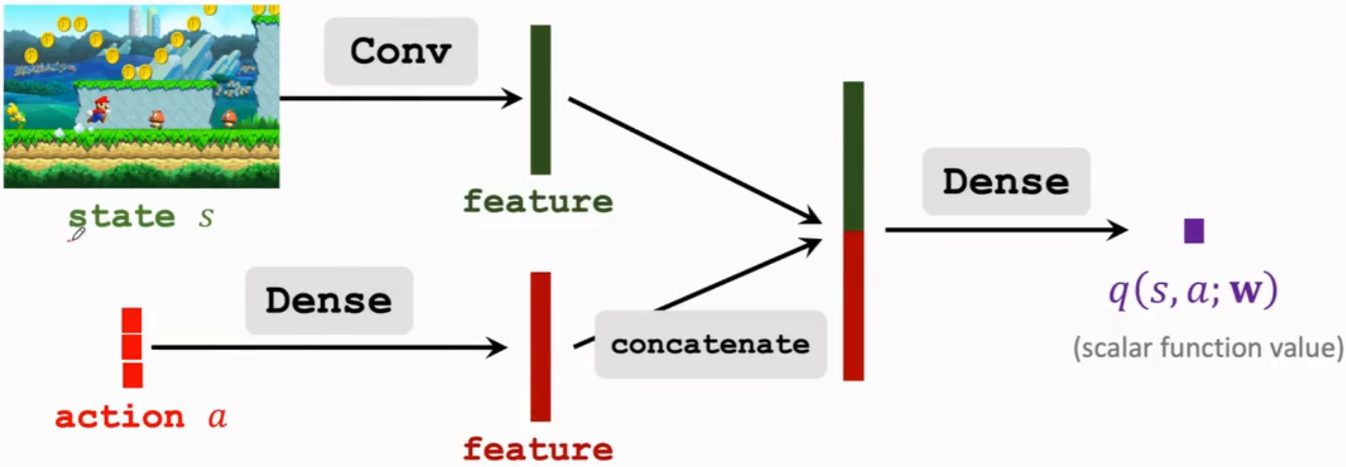
We use the neural network $Q(s,a;w)$ to approximate $Q^*(s,a)$, where w is the parameter to approximate, s is the input, and a is the output that scores all actions.

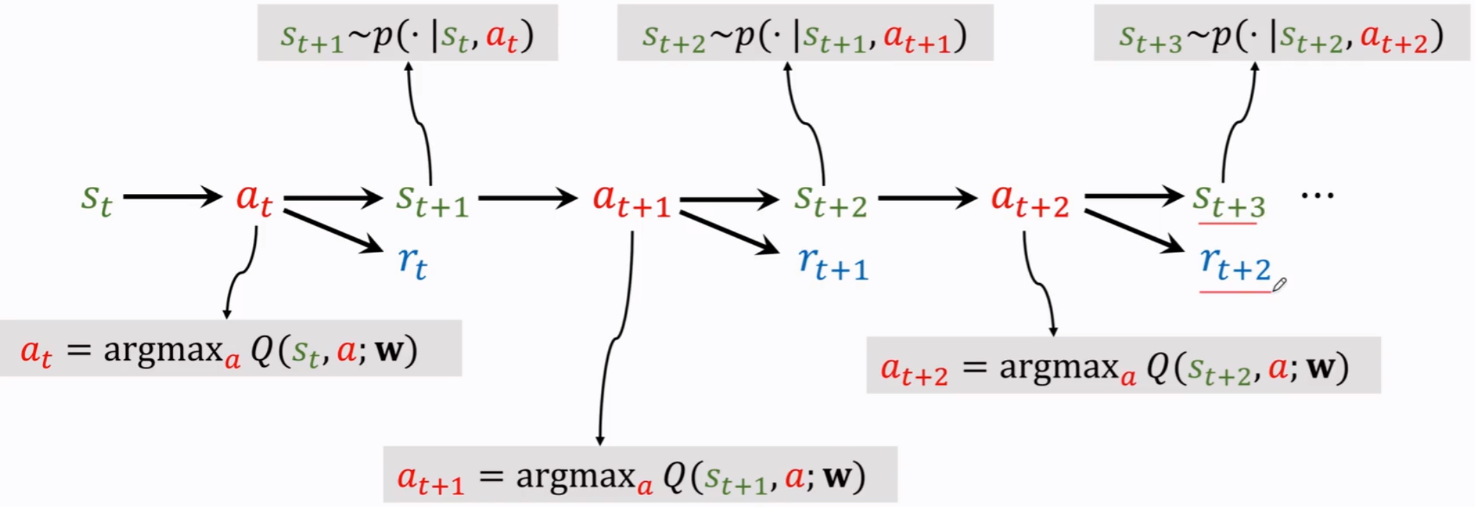
Given the currently observed state $s_t$, DQN takes $s_t$ as input, scores all actions, and selects the action with the highest score as $a_t$.

After the agent performs action $a_t$, the environment changes. The state transition function $p$ randomly samples a new state $s_{t+1}$, and the environment also tells us a return $r_t$. This $r_t$ is the key to training DQN.

(2) How to Train DQN

The conventional network training process is as follows:

1. First, make a prediction of the task outcome $q=Q(w)$
2. Obtain the target $y$ after completing the task
3. Calculate the loss $L=\frac{1}{2}(q-y)^2$
4. Calculate the gradient $\frac{\partial L}{\partial w}=\frac{\partial L}{\partial q}\cdot \frac{\partial q}{\partial w}$
5. Update the parameter $w_{t+1}=w_t-\alpha \cdot\frac{\partial L}{\partial w}|_{w=w_t}$

However, this approach requires the entire task to be completed before the parameters can be updated. To begin updating the parameters after completing only part of the task, Temporal Difference Learning (TD algorithm) was introduced. The process is as follows:

1. First, make a prediction of the task outcome $q=Q(w)$
2. After performing part of the task, predict the task outcome again as $y$. At this point, $y$ includes the completed part and a prediction of the remaining part, so it is more reliable than $q$
3. Calculate the loss $L=\frac{1}{2}(q-y)^2$
4. Calculate the gradient $\frac{\partial L}{\partial w}=\frac{\partial L}{\partial q}\cdot \frac{\partial q}{\partial w}$
5. Update the parameter $w_{t+1}=w_t-\alpha \cdot\frac{\partial L}{\partial w}|_{w=w_t}$

In deep reinforcement learning, this is represented by the following equation:

$Q(s_t,a_t;w)\approx r_t+\gamma\cdot Q(s_{t+1},a_{t+1};w)$

The expected sum of future rewards is the reward that has actually been observed plus the expected future rewards at time t+1.

1. First, make the prediction $Q(s_t,a_t;w_t)$
2. Obtain the TD target $y_t=r_t+\gamma\cdot Q(s_{t+1},a_{t+1};w_t)=r_t+\gamma\cdot max_a Q(s_{t+1},a;w_t)$
3. Calculate the loss $L_t=\frac{1}{2}[Q(s_t,a_t;w)-y_t]^2$
4. Perform gradient descent $w_{t+q}=w_t-\alpha\cdot\frac{\partial L_t}{\partial w}|_{w=w_t}$

(3) Experience Replay

Previously, we used online gradient descent to update $w$, thereby reducing the TD errer $\delta_t=q_t-t_t$.

We define an experience transition as $(s_t,a_t,r_t,s_{t+1})$. The traditional approach discards each transition after using it, which wastes experience. In addition, the traditional approach ignores correlations between different experiences.

Store the most recent n transitions in a replay buffer. When new experience arrives, delete the old transition.

1. Randomly sample a transition from the buffer each time
2. Calculate the TD error
3. Calculate the gradient
4. Perform stochastic gradient descent (in practice, minibatch SGD is generally used, sampling multiple transitions at once)

Prioritized Experience Replay: To address nonuniform data, importance sampling can be used instead of uniform sampling. Sampling can be based on the TD error: the larger the error, the higher the probability that the transition will be sampled.

Learning Rate Scaling: If a transition has a high sampling probability, its learning rate should be set relatively low.

Updating the TD error: If a transition has never been used, set its TD error to the maximum value. Update the TD error while training DQN.

III. Policy Learning

The policy function $\pi(a|s)$ is a probability density function. For each given state $s$, the policy function draws an optimal action $a$ to be performed.

Ideally, we could list all states and actions and calculate the probabilities between every state and action.

In practice, however, there are countless states, so it is impossible to record the action corresponding to every state. Function approximation is therefore required. A neural network is generally used for approximation, namely the policy network $\pi(a|s;\theta)$

The state-value function $V_\pi(s_t)=E_A[Q_\pi(s_t,A)]$ can tell us whether the current situation is good or bad. When the state is known, it can also determine whether the policy is good. The better the policy, the larger $V_\pi$ is and the higher the task completion success rate. $V_\pi$ can be expressed as:

$V_\pi(s_t)=E_A[Q_\pi(s_t,A)]=\sum_a\pi(a|s_t)\cdot Q_\pi(s_t,a)$

Replace the policy function with a neural network to obtain:

$V_\pi(s_t;\theta)=\sum_a\pi(a|s_t;\theta)\cdot Q_\pi(s_t,a)$

Given state $s$, the better the policy function, the larger the value function. We can therefore consider changing the neural network parameter $\theta$ to increase $V(s;\theta)$. Based on this idea, we can take the expectation:

$J(\theta)=E_s[V(S;\theta)]$

The better the policy network, the larger $J(\theta)$ is. To change $\theta$, we use the policy gradient algorithm.

1. Observe state $s$
2. Update the policy $\theta=\theta+\beta\cdot\frac{\partial V(s;\theta)}{\partial \theta}$ using gradient ascent, because we want the value function to be as large as possible.

For discrete actions, use $\frac{\partial V(s;\theta)}{\partial \theta}=\sum_a \frac{\partial \pi(a|s;\theta)}{\partial \theta}\cdot Q_\pi(s,a)$

For continuous actions, use $\frac{\partial V(s;\theta)}{\partial \theta}=E_{A~\pi(\cdot|s;\theta)} [\frac{\partial \pi(a|s;\theta)}{\partial \theta}\cdot Q_\pi(s,a)]$

IV. Actor-Crictic

The state-value function is defined as follows:

$V_\pi(s_t)=\sum_a\pi(a|s_t)\cdot Q_\pi(s_t,a)$

Policy network (produces actions):

• Use the neural network $\pi(a|s;\theta)$ to approximate the policy function $\pi(a|s)$
• Here, $\theta$ is the parameter to train

Value network (produces evaluation criteria):

• Use the neural network $q(s,a;w)$ to approximate the value function $Q_\pi(s,a)$
• Here, $w$ is the parameter to train

Therefore, the state-value function can be written as

$V_\pi(s_t)=\sum_a\pi(a|s_t;\theta)\cdot Q_\pi(s_t,a;w)$

Training the policy network and value network simultaneously is called the Actor-Critic Method. The general steps are as follows:

1. Observe the current state $s_t$
2. According to the policy function $\pi(\cdot|s_t;\theta_t)$, randomly sample the action $a_t$
3. Perform action $a_t$ and observe the new state $s_{t+1}$ and return $r_t$
4. Update the value network parameter $w$ using the TD algorithm
5. Update the policy network parameter $\theta$ using the policy gradient algorithm

During training, the policy network and value network must be trained simultaneously, with the value network scoring the policy network. After training is complete, the value network is no longer needed; only the policy network is required to generate actions.

V. Monte Carlo Tree Search

5.1 Basic Idea

The idea behind Monte Carlo Tree Search is that people must look many steps ahead, consider every possible situation in the future, and select the optimal action to perform.

1. If I choose to perform action $a_t$ at this point
2. How will the environment’s feedback change over the coming period $s_{t+1}$
3. Based on this environmental change, I will then perform action $a_{t+1}$
4. How will the environment change at that point

If an agent can enumerate all possibilities until the task is complete, the task will certainly have a high success rate.

5.2 Process

(1) Selection

Select an action based on its score (an imagined action that is not actually performed);

First, calculate the score for every possible action $a$:

$score(a)=Q(a)+\eta\cdot\frac{\pi(a|s_t;\theta)}{1+N(a)}$

Here, $Q(a)$ is the action value calculated by Monte Carlo Tree Search $\pi(a|s_t;\theta)$ is the trained policy network; the better the action, the higher the policy score $N(a)$ is, for the given environment state $s_t$, the number of times action $a$ has been selected so far. If the same action has been explored too many times, the denominator of this term will increase.

(2) Expansion

Imagine updating the environment;

(3) Evaluation

Evaluate the state-value score $v$ and return $r$, and set the action score to $\frac{v+r}{22}$;

(4) Backup

Update the action value using the action score $\frac{v+r}{2}$:

$Q(a_t)=mean(the recorded V's)$

Average the state values of all subsequent steps.

VI. Continuous Control

In practical reinforcement learning, the action space may be discrete (for example, controlling a game character to move up, down, left, or right), or the actions may be continuous (robotic arm joint control).

For discrete control, classification can be used directly to obtain a onehot vector. Each element of the vector represents the score for performing that action, which is used to determine which action should be performed. In continuous control, however, the action space is infinite-dimensional, so this approach cannot be applied directly to continuous control.

A relatively conventional solution is to discretize the action space, but this approach also has problems. For example, for a robotic arm with 6 degrees of freedom, even if each degree of freedom is discretized into 360 points, the entire action space contains $360^6$ points. This causes the curse of dimensionality and makes training very difficult.

There are therefore two ways to implement continuous control:

• Deterministic policy network
• Stochastic policy network

6.1 Deterministic Policy Gradient (DPG)

Consider a robotic arm with only 2 degrees of freedom. The base has a motion range of (0,180), and the robotic arm has a motion range of (0,360). Therefore, the robotic arm’s action space is the continuous set $A=[0,180]\times[0,360]$, and an action is a two-dimensional vector.

DPG is an Actor-Critic method

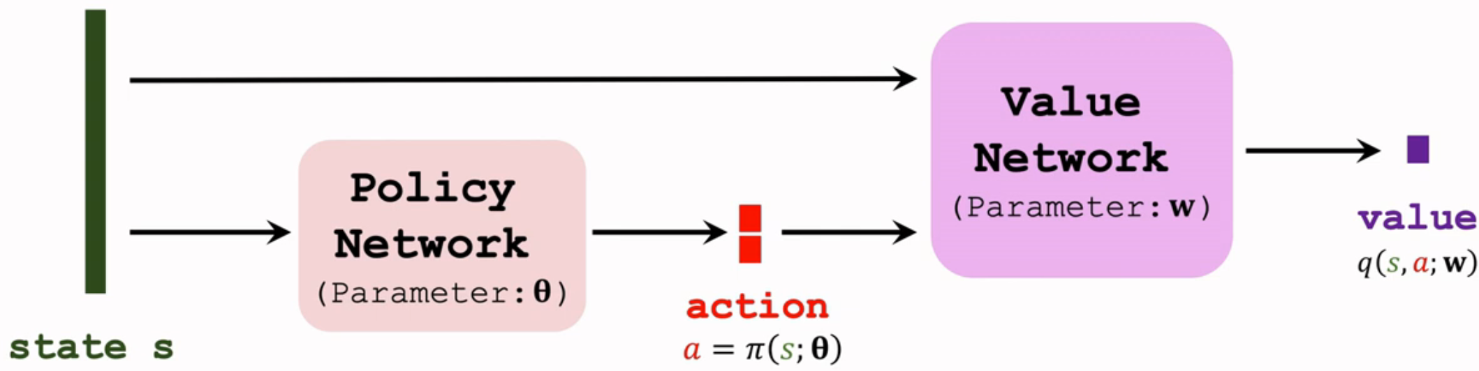
• There is a policy network that controls the agent’s motion and makes decision a based on state s; Use the policy network $a=\pi(s;\theta)$ to output a deterministic action a based on the input state s. Here, action a is the robot’s two-dimensional action vector.
• There is a value network that does not control the agent. It scores action a based on state s, thereby guiding improvements to the policy network. Use the value network $q(s,a;w)$ with state s and action a as inputs. It outputs a real number value as the evaluation of the action. The better the action, the larger the value.

The principle of DPG is therefore to train these two networks.

(1) Value Network Training

1. Obtain a training data transition $(s_t,a_t,r_t,s_{t+1})$ each time
2. Use the value network to predict the action value at the current time t: $q_t=q(s_t,a_t;w)$
3. Use the value network to predict the action value at the next time t+1: $q_{t+1}=q(s_{t+1},a_{t+1}';w)$, where $a_{t+1}'=\pi(s_{t+1};\theta)$. This action is not the action actually performed by the agent; $a_{t+1}'$ is used only to update the value network.
4. Calculate the TD error: $\delta_t=q_t-(r_t+\gamma\cdot q_{t+1})$, where the second term is the TD Target. One part is the reward actually observed, while the other part is the value network’s own prediction. Because we believe that the second term is closer to the actual situation than $q_t$ alone because it includes the real reward from this step, we want $q_t$ to approach the TD Target, which means making the TD error as small as possible.
5. Perform gradient descent to update w: $w=w-\alpha\cdot\gamma_t\cdot\frac{\partial q(s_t,a_t;w)}{\partial w}$

There is a problem here. When calculating the TD error $\delta_t=q_t-(r_t+\gamma\cdot q_{t+1})$, a bootstrapping problem can occur. That is, if the initial value is overestimated or underestimated, the TD target will also be overestimated or underestimated and will propagate back to the value network itself, causing the overestimation or underestimation to persist. The solution is to use different neural networks to calculate the TD Target, namely Target Networks.

1. Obtain a training data transition $(s_t,a_t,r_t,s_{t+1})$ each time
2. Use the value network to predict the action value at the current time t: $q_t=q(s_t,a_t;w)$
3. Use the value network to predict the action value at the next time t+1: $q_{t+1}=q(s_{t+1},a_{t+1}';w^-)$, where $a_{t+1}'=\pi(s_{t+1};\theta^-)$ $\pi(s_{t+1};\theta^-)$ is the Target policy network used in place of the policy network. Its network structure is exactly the same as the policy network, but its parameters are different. $q(s_{t+1},a_{t+1}';w^-)$ is the Target value network. It has the same structure as the value network but different parameters.

(2) Policy Network Training

Training the policy network requires the value network to evaluate how good or bad the action is, thereby guiding improvements to the policy network.

In other words, update the policy network parameter $\theta$ so that the value network considers the action $a=\pi(s;\theta)$ to be better. That is, improve $\theta$ to make the value $q(s,a;w)=q(s,\pi(s;\theta);w)$ as large as possible.

Given state s, the policy network outputs a deterministic action a, and if the value network is also deterministic, the output value is deterministic.

Therefore, the problem only requires changing $\theta$ to increase the value q. In other words, calculate the gradient of $q(s,a;w)$ with respect to $\theta$, then use gradient ascent to update $\theta$ so that $q$ increases. This gradient is called the Deterministic Policy Gradient DPG.

$$g=\frac{\partial q(s,\pi(s;\theta);w)}{\partial\theta}=\frac{\partial a}{\partial \theta}\cdot\frac{\partial q(s,a;w)}{\partial a}$$

Here, $a=\pi(s;\theta)$, then perform gradient ascent $\theta=\theta+\beta\cdot g$

The detailed steps for jointly training the policy network and value network are as follows:

1. The policy network makes a decision: $a=\pi(s;\theta)$
2. Calculate the output of the value network: $q_t=q(s,a;w)$
3. Use DPG to update the policy network: $\theta=\theta+\beta\cdot \frac{\partial a}{\partial \theta}\cdot\frac{\partial q(s,a;w)}{\partial a}$
4. Use the Target networks $\pi(s;\theta^-)$ and $q(s,a;w^-)$ to calculate $q_{t+1}$
5. Calculate the TD error: $\delta_t=q_t-(r_t+\gamma\cdot q_{t+1})$
6. Update the value network: $w=w-\alpha\cdot\gamma_t\cdot\frac{\partial q(s_t,a_t;w)}{\partial w}$
7. Update the Target networks’ parameters: $w^-=\tau\cdot w+(1-\tau)\cdot w^-$, $\theta^-=\tau\cdot \theta+(1-\tau)\cdot \theta^-$, where $\tau$ is a hyperparameter

6.2 Stochastic Policies for Continuous Control

First, consider stochastic-policy continuous control with a degree of freedom equal to 1, meaning that all actions are real numbers.

Let $\mu$ represent the mean and $\sigma$ represent the standard deviation. Both are functions of state s.

Use the probability density function of the normal distribution as the policy function:

$$\pi(a|s)=\frac{1}{\sqrt{6.28}\sigma}\cdot exp(-\frac{(a-\mu)^2}{2\sigma^2})$$

The same applies to the d-dimensional case, where the action is a d-dimensional vector.

Let vector $\mu$ represent the mean and vector $\sigma$ represent the standard deviation. Both are functions of state s.

Use a special normal distribution as the policy function:

$$\pi(a|s)=\prod_{i=1}^d\frac{1}{\sqrt{6.28}\sigma_i}\cdot exp(-\frac{(a_i-\mu_i)^2}{2\sigma^2_i})$$

However, we do not know $\mu$ and $\sigma$, so we do not know the policy function.

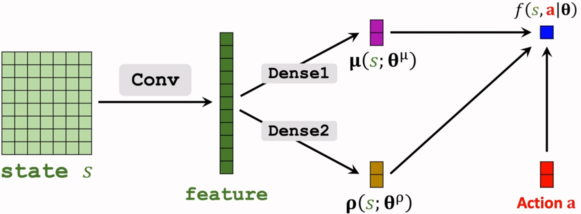
We can therefore use neural networks to approximate $\mu(s;\theta^{\mu})$ and $\rho(s;\theta{\rho})$, where $\rho_i=ln\sigma_i^2$

Take the logarithm of the policy function to turn the product into a sum, obtaining the auxiliary neural network $f(s,a;\theta)=\sum^d_{i=1}[-\frac{\rho_i}{2}-\frac{(a_i-\mu_i)^2}{2\cdot exp(\rho_i)}]$. Calculate the gradient of f with respect to the parameters in the convolutional and fully connected layers, then use it to update the parameters through backpropagation.

References:

1. Shusen Wang. Reinforcement Learning Course (YouTube)