Contents
1 What Are Multiple Convolution Kernels
1.1 Convolution
Essentially, the computation of convolution is the same as that of a fully connected layer: it is also a linear combination across neurons. The difference is that convolution selects neurons at specific positions when performing this linear combination. Below, we first use an animated diagram to get an intuitive sense of how convolution works.

As shown in the figure, **convolution is the process of taking a matrix F of a specific size each time (the shaded region in the blue matrix), sliding it across the input X (the blue matrix in the figure), and computing the inner product at each position. You can see that each time the shaded region moves one step, one convolution value is computed (the shaded region in the green matrix). After F has scanned the entire input, we obtain the full convolved result Y (the green matrix).
Meanwhile, we call this matrix F of a specific size a convolution kernel, also known as a convolutional kernel, kernel, filter, or detector. There can be one or many of them. We call the convolved result Y a feature map. Each convolution kernel produces one corresponding feature map after convolution. Finally, the shape of the input X) is represented by three dimensions: width, high, and channel. For example, in the figure the shape of input X is [7,7,1].
2.2 Multiple Convolution Kernels
Note that above I mentioned the number of convolution kernels can also be more than one. So why do we need multiple convolution kernels? In the previous article, we explained that for a single convolution kernel, we can think of it as having the ability to recognize one type of element (feature). For some complex data, relying on only one type of feature for identification is often not enough. Therefore, we usually use multiple different convolution kernels to extract features from the input and obtain multiple feature maps, and then feed them into the subsequent network.
For the same input, convolving with two different convolution kernels yields two different feature maps. From the feature maps on the right side of the figure, we can see that the upper feature map is clearly sharper than the lower one. Of course, this is also the point of using multiple convolution kernels: to detect multiple feature attributes so as to benefit downstream tasks.
3 Computing Convolution
So far, we have covered the principle and purpose of convolution, and through these animated diagrams we have gained a more intuitive understanding. But as the saying goes, without form, numbers lack intuition; without numbers, it is hard to grasp subtleties. Therefore, below we will actually compute the full convolution process using single-channel (grayscale) and three-channel inputs as examples.
3.1 Single-Channel, Single Convolution Kernel
As shown below, we now have a grayscale image of shape [5,5,1]. We need to convolve it with the convolution kernel on the right side of Figure 3, while also accounting for the effect of the bias. So what does the computation look like?
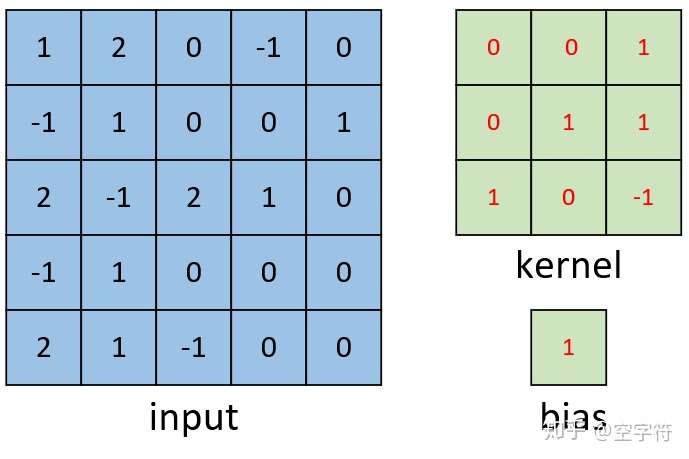
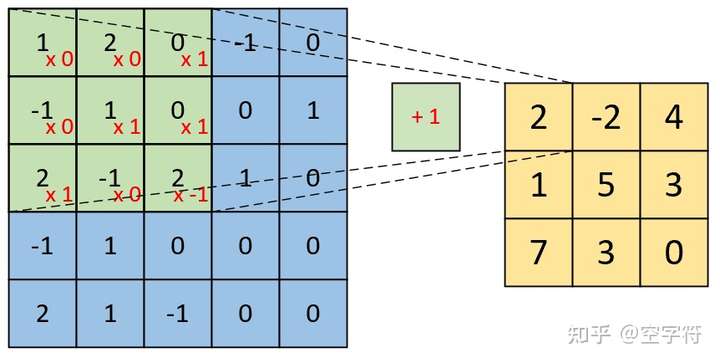
As shown below, the right side is the feature map after convolution, and the left side is a schematic of the convolution kernel convolving over the top-left of the input image. Therefore, for this part, the computation is:
Similarly, for the convolution computation at the bottom-right corner, we have:
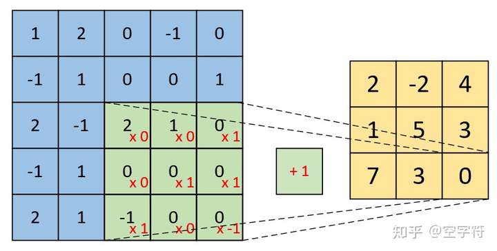
Therefore, for the final convolution result, we obtain a feature map of shape [3,3,1], as shown on the right in the figure above. That completes our introduction to single-channel, single-kernel convolution. Next, let us look at an example of single-channel, multiple-kernel convolution.
3.2 Single-Channel, Multiple Convolution Kernels
As shown below, the left side is still the input matrix. We now need to convolve it with the two convolution kernels shown on the right.
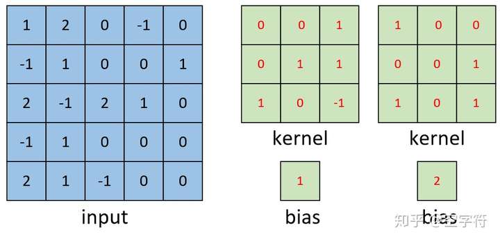
Taking the convolution kernel on the right as an example, the computation is shown below:
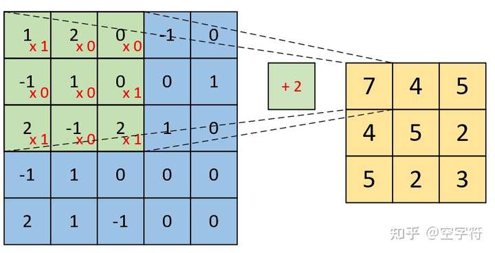
Finally, we obtain the convolved feature map on the right below, with shape [3,3,2], where 2 denotes two feature channels.
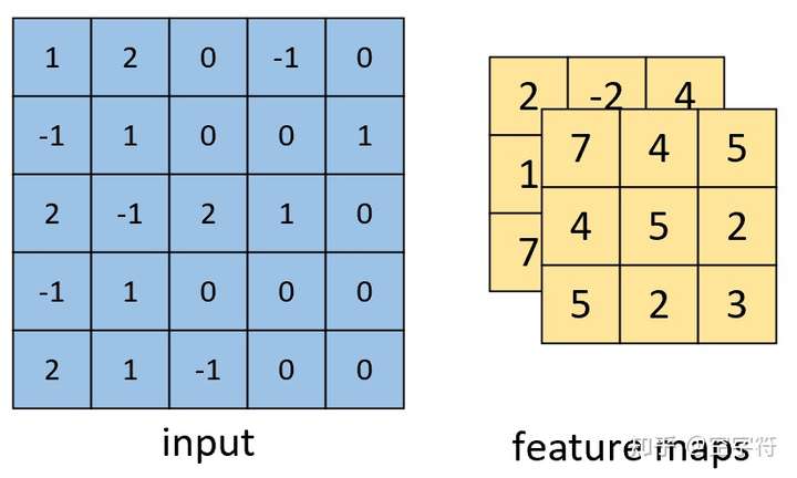
That completes the introduction to single-channel convolution computation. However, in practice we more often encounter convolution over multi-channel inputs, such as color images with RGB channels. Next, I will introduce multi-channel convolution computation.
3.3 Multi-Channel, Single Convolution Kernel
For multi-channel convolution, the overall process is still the same as before: each time we select neurons at specific positions for convolution, then move step by step until convolution is complete. Below, let us first look at multi-channel, single-kernel computation.
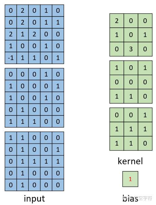
As shown in the figure, the left side is a three-channel input, and the right side shows one convolution kernel and one bias. Note: emphasize that the right side shows only one convolution kernel, not three. I have seen many people get this wrong. Because the input has three channels, each corresponding convolution kernel must also have three channels in order to perform convolution. Below, let us look at the specific computation.
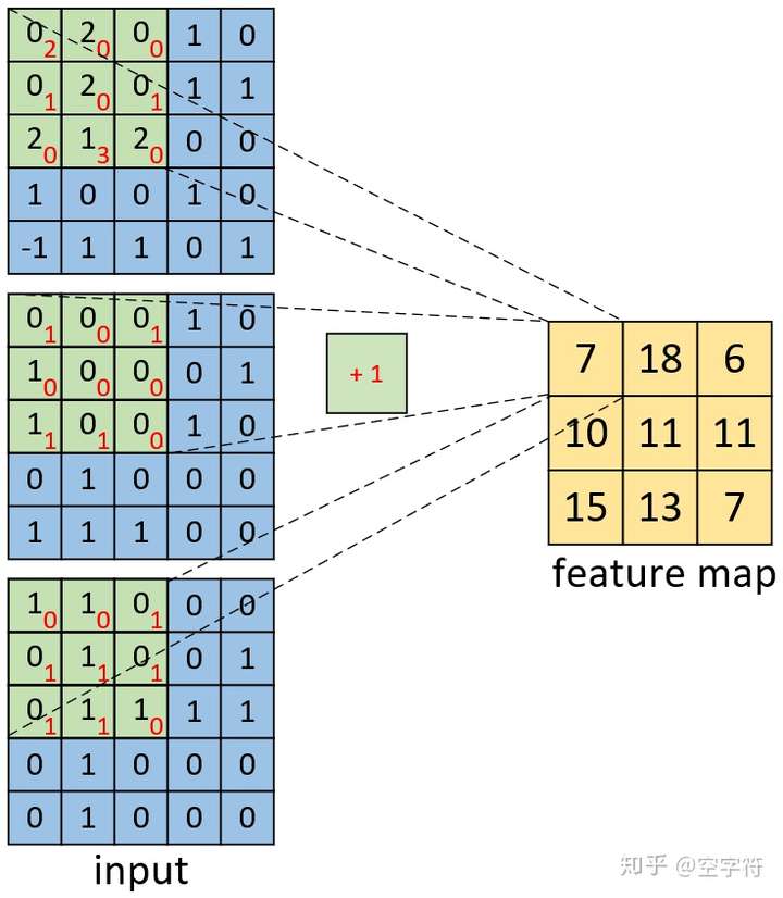
As shown in the figure, the right side is the feature map after convolution, and the left side is a schematic of a three-channel convolution kernel convolving over the top-left of the input image. Therefore, for this part, the computation is:
Similarly, the convolution computation for other regions follows steps similar to those above. From this we obtain the convolved feature map of shape [3,3,1] shown on the right in Figure 10.
3.4 Multi-Channel, Multiple Convolution Kernels
After introducing multi-channel, single-kernel computation, let us look at multi-channel, multiple-kernel computation.
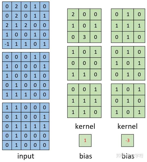
As shown in the figure, the left side is still the input matrix. We now need to convolve it with the two convolution kernels shown on the right. For the second convolution kernel, the computation is similar to equation (3): the convolution results on each channel are summed, and then the bias is added. Therefore, we finally obtain the convolved feature map of shape [3,3,2] shown on the right in Figure 12, where 2 denotes two feature channels.
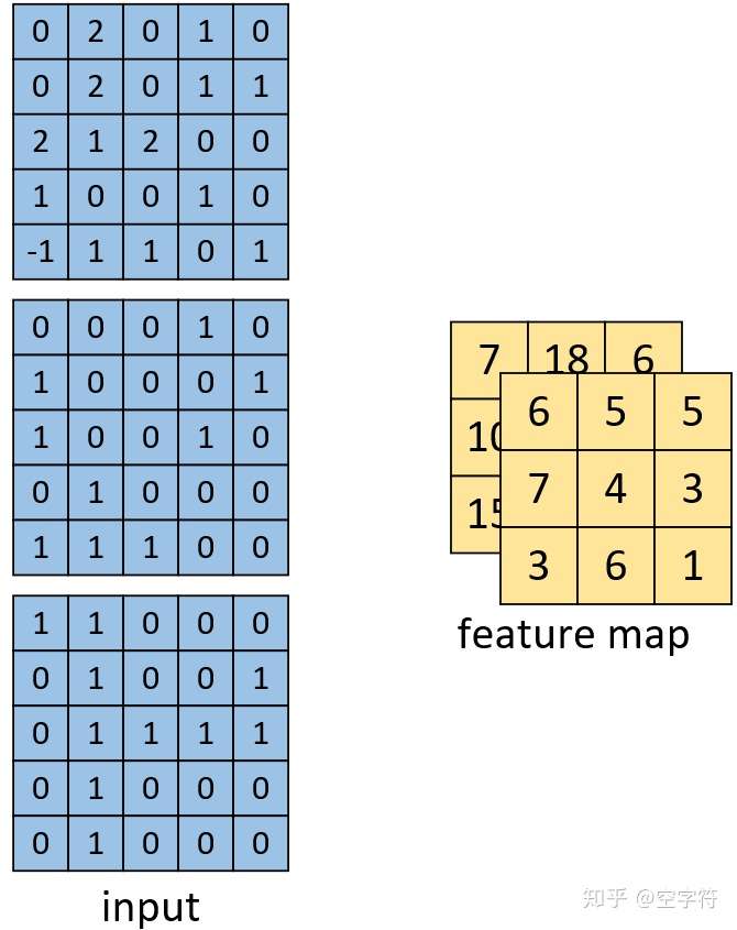
Meanwhile, from the single-channel and multi-channel convolution computations above, we can see:
(1)However many channels the original input has, one convolution kernel must have the same number of channels so that it can match the input and complete the convolution operation. In other words, if the input data has shape [n,n,c], then each convolution kernel must also have c channels.
(2)If we convolve the input with k convolution kernels, the resulting feature map will necessarily have k channels. For example, if the input is [n,n,c] and we convolve it with k kernels, then the kernel shape must be [w1,w2,c,k], and the final feature map shape must be [h1,h2,k]; here w1,w2 are the width of the convolution kernel, and h1,h2 are the width of the feature map after convolution.
Comments