Basic NumPy Methods for Data Processing

Installing NumPy

I recommend using Anaconda to manage these packages. For a detailed Anaconda tutorial, refer to the previous note, 【Basic Anaconda Usage and Calling It in PyCharm】.

After installing Anaconda, you can use activate 环境名 in Anaconda Prompt to enter an environment you created.

Use the following commands to install NumPy and Pandas:

conda install numpy
conda install pandas

Importing NumPy

import numpy as np

1. Creating Arrays

(1) Creating an Array from Existing Data

numpy.array(object, dtype = None, copy = True, order = None, subok = False, ndmin = 0)
# object  数组或嵌套的数列
# dtype   数组元素的数据类型，可选
# copy    对象是否需要复制，可选
# order   创建数组的样式，C为行方向，F为列方向，A为任意方向（默认）
# subok   默认返回一个与基类类型一致的数组
# ndmin   指定生成数组的最小维度

For example: a = np.array([[1, 2], [3, 4]]) print (a) [ [1 2] [3 4] ]

a = np.array([1, 2, 3, 4, 5], ndmin = 2) print (a) [ [1 2 3 4 5] ]

(2) Creating an Array from a Numerical Range

numpy.arange: Use the arange function to create a numerical range and return an ndarray object.

numpy.arange(start, stop, step, dtype)

The numpy.linspace function creates a one-dimensional array consisting of an arithmetic sequence.

np.linspace(start, stop, num=50, endpoint=True, retstep=False, dtype=None)
# num       要生成的等步长的样本数量，默认为50
# endpoint  该值为True时，数列中包含stop值，反之不包含，默认是True。
# retstep   如果为True时，生成的数组中会显示间距，反之不显示，默认是False

The numpy.logspace function creates a geometric sequence.

np.logspace(start, stop, num=50, endpoint=True, base=10.0, dtype=None)
# base  对数 log 的底数

(3) Creating an Array Filled with 0

numpy.zeros(shape, dtype = float, order = 'C')

(4) Creating an Array Filled with 1

numpy.ones(shape, dtype = None, order = 'C')

(5) Creating an Uninitialized Array with a Specified Shape and Data Type

numpy.empty(shape, dtype = float, order = 'C')

2. Basic Array Attributes

Attribute	Description
ndarray.ndim	Rank, meaning the number of axes or dimensions
ndarray.shape	The dimensions of the array; for a matrix, n rows and m columns
ndarray.reshape	Resizes the array
ndarray.size	The total number of array elements, equivalent to n·m in .shape
ndarray.dtype	The type of the elements in the ndarray object
ndarray.itemsize	The size of each element in the ndarray object, in bytes
ndarray.flags	Memory information for the ndarray object
ndarray.real	The real part of the ndarray elements
ndarray.imag	The imaginary part of the ndarray elements
ndarray.data	The buffer containing the actual array elements. Because elements are generally accessed by index, this attribute is usually unnecessary.

For example: a = np.array([[1,2,3],[4,5,6]]) # (2, 3)

a = np.array([[1,2,3],[4,5,6]]) b = a.reshape(3,2) print (b) [[1, 2] [3, 4] [5, 6]]

3. Array Slicing and Indexing

(1) Slicing with the slice Function

slice(start, stop[, step])
# start  起始位置
# stop   结束位置
# step   间距

(2) Slicing with Colon : Separators [start:stop:step]

a = np.arange(10) # [0 1 2 3 4 5 6 7 8 9]
b = a[2:7:2]
b = a[5]
b = a[2:]

Explanation of the colon : : If only one argument is provided, such as [2], the single element corresponding to that index is returned. [2:] means that all items from that index onward are extracted. If two arguments are used, such as [2:7], the items between the two indices are extracted, excluding the stop index.

(3) The split Method

The numpy.split function splits an array into subarrays along a specified axis.

numpy.split(ary, indices_or_sections, axis)
# ary：被分割的数组
# indices_or_sections：如果是一个整数，就用该数平均切分，如果是一个数组，为沿轴切分的位置（左开右闭）
# axis：设置沿着哪个方向进行切分，默认为 0，横向切分，即水平方向。为 1 时，纵向切分，即竖直方向

4. Basic Array Operations

(1) Flattening an Array

numpy.ndarray.flatten returns a copy of an array. Changes made to the copy do not affect the original array.

a = np.arange(8).reshape(2,4)
a.flatten()             # [0 1 2 3 4 5 6 7]
a.flatten(order = 'F')  # [0 4 1 5 2 6 3 7]
# order：'C'按行，'F'按列，'A'原顺序，'K'元素在内存中的出现顺序

numpy.ravel() flattens the array elements, usually in “C-style” order, and returns an array view (view, somewhat similar to the meaning of a C/C++ reference). Changes affect the original array.

a = np.arange(8).reshape(2,4)
a.ravel()              # [0 1 2 3 4 5 6 7]
a.ravel(order = 'F')  # [0 4 1 5 2 6 3 7]

(2) Transposing an Array

numpy.transpose(arr, axes)
# arr ：要操作的数组
# axes：整数列表，对应维度，通常所有维度都会对换

numpy.T
# 数组全部转置

For example: a = np.arange(12).reshape(3,4) print (np.transpose(a)) print (a.T)

(3) Moving and Swapping Array Axes

The numpy.rollaxis function moves a specified axis to a specified position.

numpy.rollaxis(arr, axis, start)
# arr   ：数组
# axis  ：要移动的轴，其它轴的相对位置不会改变
# start ：默认为零，表示完整的滚动。会滚动到特定位置

The numpy.swapaxes function swaps two axes of an array.

numpy.swapaxes(arr, axis1, axis2)
# arr   ：数组
# axis1 ：对应第一个轴的整数
# axis2 ：对应第二个轴的整数

(4) Joining Arrays

Array Concatenation

numpy.concatenate((a1, a2, ...), axis)
# a1, a2, ... ：相同类型的数组
# axis：沿着它连接数组的轴，默认为 0

For example: a = np.array([[1,2],[3,4]]) b = np.array([[5,6],[7,8]]) print (np.concatenate((a,b))) [[1 2] [3 4] [5 6] [7 8]] print (np.concatenate((a,b),axis = 1)) [[1 2 5 6] [3 4 7 8]]

Array Stacking

The numpy.stack function joins a sequence of arrays along a new axis.

numpy.stack(arrays, axis)
# arrays : 相同形状的数组序列
# axis   : 返回数组中的轴，输入数组沿着它来堆叠

For example: a = np.array([[1,2],[3,4]]) b = np.array([[5,6],[7,8]]) print (np.stack((a,b),0)) [[[1 2] [3 4]] [[5 6] [7 8]]] print (np.stack((a,b),1)) [[[1 2] [5 6]] [[3 4] [7 8]]]

For specific array-stacking methods, refer to this article: 【The Most Intuitive and Easy-to-Understand Explanation of the numpy.stack() Function in Python】

(5) Changing an Array’s Shape

numpy.resize

The numpy.resize function returns a new array of the specified size. If the new array is larger than the original, it contains copies of the elements from the original array.

numpy.resize(arr, shape)
# arr   : 要修改大小的数组
# shape : 返回数组的新形状

(6) Operating on Array Elements

numpy.append

The numpy.append function adds values to the end of an array. The append operation allocates the entire array and copies the original array into the new array. In addition, the dimensions of the input arrays must match; otherwise, a ValueError is generated.

numpy.append(arr, values, axis=None)
# arr   ：输入数组
# values：要向arr添加的值，需要和arr形状相同（除了要添加的轴）
# axis  ：默认为 None。当axis无定义时，是横向加成，返回总是为一维数组！当axis有定义的时候，分别为0和1的时候。当axis有定义的时候，分别为0和1的时候（列数要相同）。当axis为1时，数组是加在右边（行数要相同）。

numpy.insert

The numpy.insert function inserts values into an input array before a given index along a given axis.

numpy.insert(arr, obj, values, axis)
# arr   ：输入数组
# obj   ：在其之前插入值的索引
# values：要插入的值
# axis  ：沿着它插入的轴，如果未提供，则输入数组会被展开

numpy.delete

The numpy.delete function returns a new array with a specified subarray removed from the input array.

numpy.delete(arr, obj, axis)
# arr ：输入数组
# obj ：可以被切片，整数或者整数数组，表明要从输入数组删除的子数组
# axis：沿着它删除给定子数组的轴，如果未提供，则输入数组会被展开

numpy.unique

The numpy.unique function removes duplicate elements from an array.

numpy.unique(arr, return_index, return_inverse, return_counts)
# arr：输入数组，如果不是一维数组则会展开
# return_index：如果为true，返回新列表元素在旧列表中的位置（下标），并以列表形式储
# return_inverse：如果为true，返回旧列表元素在新列表中的位置（下标），并以列表形式储
# return_counts：如果为true，返回去重数组中的元素在原数组中的出现次数

(7) Sorting an Array

Type	Speed	Worst Case	Workspace	Stability
'quicksort' (quick sort)	1	O(n^2)	0	No
'mergesort' (merge sort)	2	O(n*log(n))	~n/2	Yes
'heapsort' (heap sort)	3	O(n*log(n))	0	No

numpy.sort()

The numpy.sort() function returns a sorted copy of the input array.

numpy.sort(a, axis, kind, order)
# a: 要排序的数组
# axis: 沿着它排序数组的轴，如果没有数组会被展开，沿着最后的轴排序， axis=0 按列排序，axis=1 按行排序
# kind: 默认为'quicksort'（快速排序）
# order: 如果数组包含字段，则是要排序的字段

a = np.array([[3,7],[9,1]])
print (np.sort(a))  # [[3 7],[1 9]]
print (np.sort(a, axis = 0))  # [[3 1],[9 7]]

numpy.argsort()

The numpy.argsort() function returns the indices that would sort the array values in ascending order.

np.argsort([3, 1, 2])  # [1 2 0]

(8) Array Multiplication

numpy.dot()

 numpy.dot(a, b, out=None): For two-dimensional arrays, it is equivalent to matrix multiplication; for one-dimensional arrays, it is the inner product of vectors; for n-dimensional arrays, it is the sum product over the last axis of a and the second-to-last axis of b.

>>> np.dot(3, 4)
12
>>> np.dot([2, 3], [4, 4])
20

>>> a = [[1, 0], [0, 1]]
>>> b = [[4, 1], [2, 2]]
>>> np.dot(a, b)
array([[4, 1], [2, 2]])

numpy.outer()

numpy.outer(a, b, out=None): Computes the outer product of two vectors. If the inputs a,b are not one-dimensional arrays, they are first converted to one-dimensional arrays, giving a(M,) and b(N,), and producing an output with shape (M,N).

[[a0*b0 a0*b1 ... a0*bN ]
 [a1*b0 .               ]
 [ ... .                ]
 [aM*b0           aM*bN ]]

numpy.multiply()

numpy.multiply(a, b): Computes the element-wise product. It can only be used when the dimensions are equal. When the dimensions of the arrays or matrices being multiplied differ, they are expanded to a consistent form according to certain broadcasting rules.

*

*: When two arrays are multiplied, this works the same way as np.multiply and computes the element-wise product. However, when the multiplied elements are matrices, it works the same way as np.dot and represents matrix multiplication.

5. Broadcast Rules

Broadcasting is how numpy performs numerical calculations on arrays with different shapes. Arithmetic operations on arrays are usually performed on corresponding elements.

The specific broadcasting rules are as follows:

• Align all input arrays with the array having the longest shape, filling any missing parts of a shape by adding 1 at the front.
• The shape of the output array is the maximum value along each dimension of the input-array shapes.
• If the length of a dimension in an input array is the same as the length of the corresponding dimension in the output array, or if its length is 1, the array can be used in the calculation; otherwise, an error occurs.
• When the length of a dimension in an input array is 1, operations along that dimension use the first set of values on that dimension.

Example:

a = np.array([[ 0, 0, 0],
           [10,10,10],
           [20,20,20],
           [30,30,30]])
b = np.array([1,2,3])
print(a + b)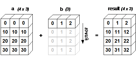

6. Basic Array Computations

(1) Arithmetic Functions

Addition, Subtraction, Multiplication, and Division

NumPy arithmetic functions include simple addition, subtraction, multiplication, and division: add(), subtract(), multiply(), and divide(). The arrays must have the same shape or conform to the array broadcasting rules.

a = np.arange(9, dtype = np.float_).reshape(3,3)
b = np.array([10,10,10])
print (np.add(a,b))
print (np.subtract(a,b))
print (np.multiply(a,b))
print (np.divide(a,b))

Reciprocal

The numpy.reciprocal() function returns the element-wise reciprocal of its argument.

a = np.array([0.25, 1.33, 1, 100])
print (np.reciprocal(a))

Power

The numpy.power() function uses the elements in the first input array as bases and raises them to the powers of the corresponding elements in the second input array.

a = np.array([10,100,1000])
b = np.array([1,2,3])
print (np.power(a,b))

Modulus and Remainder

numpy.mod() calculates the remainder after dividing corresponding elements in the input arrays. The numpy.remainder() function produces the same result.

a = np.array([10,20,30])
b = np.array([3,5,7])
print (np.mod(a,b))
print (np.remainder(a,b))

(2) Statistical Functions

Maximum and Minimum

numpy.amin() calculates the minimum values of the elements in an array along a specified axis. numpy.amax() calculates the maximum values of the elements in an array along a specified axis. The numpy.argmax() and numpy.argmin() functions return the indices of the maximum and minimum elements, respectively, along a given axis.

a = np.array([[3,7,5],[8,4,3],[2,4,9]])
print (np.amin(a,1))    # [3 3 2]
print (np.amin(a,0))    # [2 4 3]
print (np.amax(a))      # 9
print (np.amax(a, axis = 0))   # [8 7 9]
print (np.argmax(a))    # 8
print (np.argmax(a, axis = 0)) # [1 0 2]
print (np.argmin(a))    # 6
print (np.argmin(a, axis = 1)) # [0 2 0]

Range (Maximum - Minimum)

The numpy.ptp() function calculates the difference between the maximum and minimum values of the elements in an array (maximum - minimum).

a = np.array([[3,7,5],[8,4,3],[2,4,9]])
print (np.ptp(a))    # 7
print (np.ptp(a, axis = 1))    # [4 5 7]
print (np.ptp(a, axis = 0))    # [6 3 6]

Arithmetic Mean

The numpy.mean() function returns the arithmetic mean of the elements in an array. If an axis is provided, it computes the mean along that axis.

a = np.array([[1,2,3],[3,4,5],[4,5,6]])
print (np.mean(a))    # 3.6666666666666665
print (np.mean(a, axis = 0))  # [2.66666667 3.66666667 4.66666667]
print (np.mean(a, axis = 1))  # [2. 4. 5.]

Weighted Average

The numpy.average() function computes the weighted average of the elements in an array using their respective weights given in another array.

a = np.array([1,2,3,4])
print (np.average(a))  # 2.5
wts = np.array([4,3,2,1])
print (np.average(a,weights = wts))  # 2.0

Median

The numpy.median() function calculates the median (middle value) of the elements in array a.

a = np.array([[30,65,70],[80,95,10],[50,90,60]])
print (np.median(a))  # 65.0
print (np.median(a, axis = 0))  # [50. 90. 60.]
print (np.median(a, axis = 1))  # [65. 80. 60.]

Variance

In statistics, variance (sample variance) is the mean of the squared differences between each sample value and the mean of all sample values, namely mean((x - x.mean())** 2).

np.var([1,2,3,4])  # 1.25

Standard Deviation

Standard deviation measures how dispersed a set of data is around its mean and is the arithmetic square root of the variance.

np.std([1,2,3,4])  # 1.1180339887498949