[Object Recognition] SIFT Algorithm: Theory

I. Introduction

1.1 The SIFT Algorithm

SIFT (Scale-Invariant Feature Transform) is an algorithm for detecting and describing local image features. The algorithm searches for extrema across scale space and extracts position, scale, and rotation invariants. These keypoints remain stable under changes in illumination, affine transformation, and noise.

1.2 How SIFT Features Are Obtained

1. Scale-space extrema detection

   Use the Difference-of-Gaussians function to search across all scales and image locations, finding candidate keypoints that are invariant to scale and orientation.

2. Keypoint localization

   For each candidate keypoint, determine its position and scale and ensure its stability.

3. Orientation assignment

   Assign one or more orientations to each keypoint based on local image gradient directions.

4. Keypoint description

   Measure local image gradients in a selected scale around each keypoint. This information captures allowable local shape distortion and illumination variation.

1.3 Image Matching and Recognition

1. Extract SIFT features from a set of reference images of target objects and store them in a database.
2. Compare each feature in a new image against the database one by one, finding matching features by Euclidean distance between feature vectors.

1.4 How to Improve Matching Accuracy

1. By using a subset of keypoints whose position, scale, and orientation are consistent with the object in the new image, correct matches can be filtered from the match set. Using several features together as evidence yields a far lower error rate than matching on a single feature alone.

2. Matching methods

   ① First perform a least-squares estimate of a radiation approximation of the object pose. Other image features consistent with this pose are identified, and outliers are discarded.

   ② Given the accuracy of you and and the number of possible incorrect matches, compute in detail the probability that a set of features indicates the presence of an object.

   ③ Object matches that pass all tests can be labeled as correct with high confidence.

II. Scale-Space Extrema Detection

The SIFT algorithm finds keypoints across different scale spaces. Obtaining scale space requires Gaussian blur.

2.1 Gaussian Blur

(1) The Gaussian Function

Gaussian blur uses a Gaussian function (normal distribution) to compute a blur kernel and convolves that kernel with the original image to blur it.

Gaussian formula in N-dimensional space:

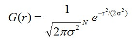
• $\sigma$ is the standard deviation of the normal distribution; the larger $\sigma$ is, the more blurred and smoother the image becomes
• $r$ is the blur radius, the distance from a kernel element to the kernel center

Gaussian formula in two-dimensional space:

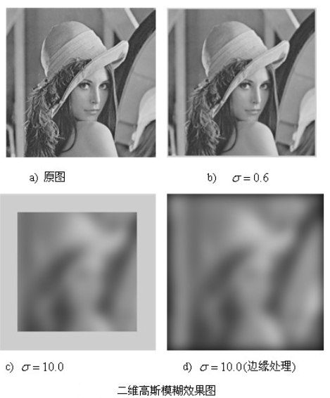
• $\sigma$ is the standard deviation of the normal distribution; the larger $\sigma$ is, the more blurred and smoother the image becomes
• m,n are the dimensions of the two-dimensional kernel, m×n
• x,y are the coordinates of an element on the kernel (x,y)

The surface generated by a two-dimensional Gaussian function is a set of concentric circles of normal distribution starting from the center. Each pixel value is a weighted average of surrounding neighboring pixels. The original pixel has the greatest weight, and edge pixels have progressively smaller weights, so edges are preserved more effectively.

When computing the discrete approximation for each pixel, pixels beyond $3\sigma$ can be treated as having no effect. Therefore, image processing programs only need to compute a $(6\sigma+1)\times(6\sigma+1)$ matrix.

(2) Two-Dimensional Gaussian Blur

Compute the Gaussian kernel matrix from $\sigma$ (with size $(6\sigma+1)\times(6\sigma+1)$, values computed from $G(x,y)$)

Normalize the Gaussian kernel matrix (ensuring matrix elements fall within $[0,1]$). For example, the $5\times5$ Gaussian kernel below shows that the Gaussian kernel is center-symmetric.

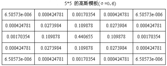
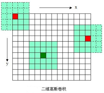
Convolve this Gaussian kernel matrix with the original image to obtain the Gaussian-blurred image. The convolution process is illustrated below:

(3) Separable Gaussian Blur

Two-dimensional Gaussian blur has two shortcomings:

1. Using two-dimensional Gaussian blur causes edge pixels to be lost; the larger $\sigma$ is, the more pixels are lost
2. As the kernel grows, the computational cost of Gaussian kernel convolution increases sharply

Solution:

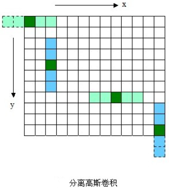
Exploit the separability of the Gaussian function (the effect of a two-dimensional matrix transform is equivalent to a horizontal one-dimensional Gaussian matrix transform followed by a vertical one-dimensional Gaussian matrix transform).

1. Two passes of one-dimensional Gaussian convolution eliminate the edge artifacts produced by the two-dimensional Gaussian matrix.
2. Convolution requires only O(n×M×N)+O(m×M×N) operations, whereas the two-dimensional matrix requires O(m×n×M×N) operations. Here m,n are the dimensions of the Gaussian matrix. M,N are the dimensions of the two-dimensional image.

2.2 Scale Space

(1) The Concept of Scale Space

1. Concept

   Introduce a parameter treated as scale into the image information processing model. By continuously varying the scale parameter, obtain a multi-scale scale-space representation sequence. Extract the main contours of scale space from these sequences and use those main contours as feature vectors to achieve edge and corner detection and feature extraction at different resolutions.

2. Characteristics

   Incorporate traditional single-scale image information processing techniques into a dynamic analysis framework in which scale changes continuously. Essential image features are easier to obtain. Images at each scale in scale space become progressively more blurred, simulating how a target forms on the retina as distance increases from near to far.

3. Advantages

   1）Scale-space operators are unaffected by changes in image gray level and contrast, satisfying gray-level invariance and contrast invariance;

   2）Scale-space operators are independent of image position, size, angle, and affine transformation, satisfying translation invariance, scale invariance, Euclidean invariance, and affine invariance.

(2) Representing Scale Space

Scale space $L(x,y,z)$ is defined as the convolution of a Gaussian function $G(x,y,\sigma)$ with varying scale and the original image $I(x,y)$.

Here $\sigma$ is the scale factor. The smaller $\sigma$ is, the less blur is applied, and the corresponding scale is smaller. Therefore, large scales correspond to coarse image features, and small scales correspond to fine image details.

(3) Building a Gaussian Pyramid

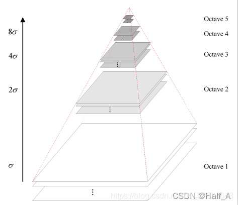
Scale space is represented using a Gaussian pyramid in practice. Building a Gaussian pyramid involves two steps: 1）downsampling the image; and 2）applying Gaussian smoothing to the image.

A pyramid model repeatedly downsamples the original image to obtain a series of images of different sizes, from large to small and from bottom to top. The original image is the first layer of the pyramid; each downsampling step produces a new pyramid layer. To make scale continuity explicit, the Gaussian pyramid adds Gaussian filtering on top of simple downsampling.

As shown in the figure above, each image in a pyramid layer is Gaussian-blurred with different parameters. Octave denotes the number of image groups that can be produced from one image, and Interval denotes the number of image layers in one group. In addition, during downsampling, the initial image (bottom image) of each group in the Gaussian pyramid is obtained by subsampling the third-to-last image of the previous group.

Layer count for the Gaussian pyramid:

M,N: original image dimensions t: logarithm of the minimum dimension of the top-of-pyramid image

2.4 Extrema Detection Method

Because extrema must be found in scale space, adjacent upper and lower layers within each group of the Gaussian pyramid are subtracted in practice to obtain Difference-of-Gaussian (DOG) images for extrema detection. That is, the difference between two adjacent scales (with constant k distinguishing adjacent scales):

$D(x, y, σ) = (G(x, y, kσ)−G(x, y, σ))∗I(x, y)$

​ $=L(x, y, kσ)−L(x, y, σ)$

To find extrema of the Difference-of-Gaussian function, each pixel is compared with all of its neighbors to determine whether it is larger or smaller than its neighbors in the image domain and scale domain. As shown in the figure, the center detection point is compared with 8 neighbors at the same scale and with 9×2 points on adjacent scales above and below, for a total of 26 points, ensuring that extrema are detected in both scale space and two-dimensional image space.

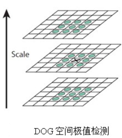
Because comparison across adjacent scales is required, within each group of the DOG pyramid, extrema can only be detected on the middle layers; the top and bottom layers cannot be used.

To detect S extrema at S scales within each group, each DOG pyramid group needs S+2 image layers. Because the DOG pyramid is obtained by subtracting adjacent layers of the Gaussian pyramid, each Gaussian pyramid group needs S+3 image layers. In practice, S is between 3 and 5.

2.5 Sampling Frequency for Extrema Detection

To detect local maxima and minima, select among 8 neighboring points on the same layer as the sample and 9 neighboring points on each of the adjacent layers above and below. A point is an extremum only if it is greater than or all of these neighboring points. After detection, the vast majority of sample points are discarded.

An important question is determining the sampling frequency in image and scale space to detect extrema reliably. In practice, extrema can lie very close together, so a solution that balances efficiency and completeness is needed.

(1) Sampling Frequency in the Scale Domain

From extensive experimental data:

（1）When more scales are sampled, repeatability does not continue to improve, because more local extrema are detected, but on average these extrema are less stable and less likely to be detected in transformed images.

（2）As sampling density increases, the number of keypoints increases and the total number of correct matches increases. Because object recognition success in practice depends more on the number of correctly matched keypoints than on the percentage of correct matches, using a large number of samples is best. However, this increases computational cost, so Lowe recommends using 3 scale samples per group

(2) Sampling Frequency in the Spatial Domain

The sampling frequency in the image domain within one scale must be determined. If extrema can lie arbitrarily close together, a similar trade-off exists between spatial sampling frequency and detection rate. Here Lowe recommends, based on experiments, using $\sigma=1.6$.

Because differencing is performed before extrema detection, the highest spatial frequencies are discarded. To make full use of the input, the input image can be doubled in size using linear interpolation before building the first level of the pyramid.

III. Keypoint Localization

3.1 Accurate Keypoint Localization

Extrema in discrete space are not the true extrema of the image.

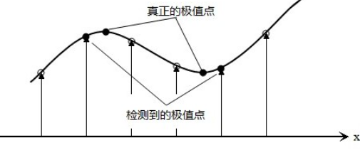
To improve keypoint stability, curve fitting is applied to the scale-space function. Using the Taylor expansion of the scale-space function, the derivative is 0 at an extremum, and the offset of $x$ is solved to localize the keypoint precisely.

Taylor-expand the scale-space function $D(x,y,\sigma)$ with the origin coinciding with the sample point.

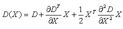
Differentiate $D(x,y,\sigma)$ and set the result to zero. Solving yields $\hat{x}=−\frac{∂^2D^{-1}}{∂x^2}\frac{∂D}{∂x}$, which is the offset of $x$.

3.1 Eliminating Edge Responses

For stability, removing low-contrast keypoints alone is not enough; edge responses introduced by the Difference-of-Gaussian function must also be eliminated. Along the edge gradient direction, the principal curvature is large; perpendicular to the edge (along the edge direction), the principal curvature is small. Principal curvatures can be computed from the Hessian matrix:

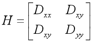
Its eigenvalues are proportional to the principal curvatures of D. Because only the ratio $r$ of the eigenvalues is needed, the eigenvalues themselves need not be computed. Let $\alpha$ be the larger eigenvalue and $\beta$ the smaller eigenvalue. Take $\alpha=r\beta$. Using properties of the trace and determinant:

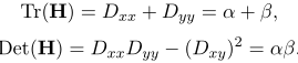
Therefore, when the two eigenvalues are equal, the expression $\frac{Tr(H)^2}{Det(H)}=\frac{(r+1)^2}{r}$ has its minimum value, and this expression increases as the ratio $r$ increases. To test whether the principal curvature is below a certain threshold, it suffices to test

$\frac{Tr(H)^2}{Det(H)}<\frac{(r+1)^2}{r}$. Retain the feature point when this condition is met; otherwise discard it. (Commonly T=1.2)

IV. Gradient Orientation Assignment

4.1 Gradient Magnitude and Direction

To make keypoint descriptors rotation invariant, assign each keypoint a reference orientation using local image features so that descriptors are invariant to image rotation. For keypoints detected in the Difference-of-Gaussian pyramid, collect gradient magnitude and orientation distribution features of pixels in a $3\sigma$ neighborhood window on the corresponding Gaussian pyramid image. Gradient magnitude and direction are as follows:

4.2 Gradient Statistics

After computing keypoint gradients, use a histogram to tabulate the gradients and orientations of pixels in the neighborhood. The gradient histogram divides the 0~360° range into 36 bins, each representing a 10° range. As shown in the figure, the peak of the histogram represents the keypoint’s principal orientation.

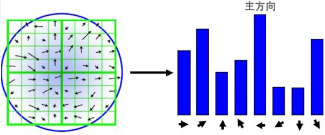
Use the maximum value in the histogram as the keypoint’s principal orientation. To improve matching robustness, retain only orientations whose peak exceeds 80％ of the principal-orientation peak as secondary orientations for the keypoint.

V. Keypoint Descriptors

After the steps above, each keypoint has position, scale, and orientation.

The next step is to build a descriptor for each keypoint: represent the keypoint with a vector so that it remains unchanged under various transformations, including illumination and viewpoint changes.

5.1 Descriptor Representation

(1) Feature Vector Representation

First sample image gradient magnitude and orientation around each keypoint, choosing the degree of Gaussian blur based on the keypoint’s scale. To achieve orientation invariance, descriptor coordinates and gradient directions are rotated relative to the keypoint orientation.

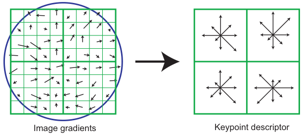
Use a Gaussian weighting function with $\sigma$ equal to half the sub-window width to weight each sample point. (This avoids sudden changes in the descriptor caused by small shifts in window position and reduces the influence of gradients far from the descriptor center, which are most likely to be matched incorrectly.)

The descriptor is a vector of all orientation-histogram bin values. Lowe’s experiments showed that the best choice is: divide each keypoint into 4 sub-regions, corresponding to 4 descriptors, each using a 4x4 array of orientation histograms with 8 gradient directions per histogram. Therefore each keypoint uses 4x4x8=128 feature values.

(2) Normalization

Adjust the feature vector to reduce the effect of illumination changes.

1. Eliminating contrast effects

Because a change in image contrast multiplies each pixel value by a constant, normalization eliminates the effect of contrast.

Therefore, first normalize the vector to unit length.

2. Eliminating illumination effects

Image brightness adds a constant to each pixel, so brightness changes do not affect image gradients. Therefore the descriptor is invariant to affine illumination changes. (Nonlinear illumination is not considered.)

To account for illumination variation, threshold the unit feature vector so that no component exceeds 0.2 (determined experimentally by Lowe), reducing the influence of large gradients, then renormalize. At this point matching large gradients is no longer as important; the distribution of orientations matters more.

VI. Application to Object Recognition

Object recognition is first performed by matching each keypoint independently against a keypoint database extracted from training images. Because of ambiguous features and background effects, initial matches are necessarily inaccurate. Therefore clusters of at least three features must first be identified; these clusters are consistent with object pose, and their correctness is far higher than that of a single-feature match. Then perform a geometric fit check on each cluster and accept or reject based on the fit result.

1. From the training images, identify the nearest neighbors in the keypoint database and find the best candidate match for each keypoint. (Nearest neighbors can use minimum Euclidean distance.)
2. Discard image features that have no correct match in the database.
3. If there are multiple match results, define the second nearest neighbor as known to come from a different object. Many other incorrect matches may lie at similar distances. The second-nearest match can be treated as providing an estimate of incorrect-match density in this region of feature space.

VII. Summary

SIFT features are stable and invariant, and play an important role in image processing and computer vision.

Main steps of the SIFT algorithm

1. Scale-space extrema detection

2. Keypoint localization

3. Orientation assignment

4. Keypoint description and matching