[Deep Learning Notes 02] Implementation of Data Operations and Linear Algebra Fundamentals

I. Data Operations and Data Preprocessing

1.1 Data Operations

(1) N-dimensional arrays

0-dimensional, a scalar representing a single category

1.0

1-dimensional, a vector representing a feature vector

[1.0, 2.7, 3.4]

2-dimensional, a matrix representing a sample or feature matrix

[[1.0, 2.7, 3.4]
 [5.0, 0.2, 4.6]
 [4.3, 8.5, 0.2]]

3-dimensional, representing an RGB image (width × height × channels)

[[[1.0, 2.7, 3.4]
  [5.0, 0.2, 4.6]
  [4.3, 8.5, 0.2]]
 [[3.2, 5.7, 3.4]
  [5.4, 6.2, 3.2]
  [4.1, 3.5, 6.2]]]

4-dimensional, representing a batch of videos or RGB images (batch size × width × height × channels)

[[[[...
	...
	...]]]]

5-dimensional, representing a batch of videos (batch size × time × width × height × channels)

[[[[[...
	 ...
	 ...]]]]]

(2) Array-related concepts

Creating an array requires

1. shape
2. data type of each element
3. value of each element

Accessing elements

1. a single element: [1, 2]
2. a row: [1, :]
3. a column: [:, 1]
4. a subregion: [1:3, 1:]
5. strided access: [::3, ::2]

1.2 Implementing Data Operations

(1) Import torch

import torch

(2) Create tensors

x = torch.arange(10)
# 输出：tensor([0, 1, 2, 3, 4, 5, 6, 7, 8, 9, 10, 11])

(3) Get the shape of a tensor

x.shape
# 输出：torch.Size([12])

(4) Get the number of elements in a tensor

x.numel()
# 输出：12

(5) Reshape a tensor

X = x.reshape(3, 4)

Note: reshape only creates a shallow copy. For example, a = torch.arange(6) b = a.reshape((2,3)) b[:]=2 After this operation, a also becomes tensor([2, 2, 2, 2, 2, 2]) Essentially, b creates a view of a—it observes a in a particular way, and they still share the same memory space.

(6) Create and initialize matrices

torch.zeros((2, 3, 4))
torch.ones(2, 3, 4)

(7) Convert a list to a tensor

torch.tensor(list)

(8) Standard tensor operators are element-wise

x = torch.tensor([1.0, 2, 4, 8])
y = torch.tensor([2, 2, 2, 2])
x + y
x - y
x * y
x / y
x ** y

(9) Concatenate multiple tensors

X = torch.arange(12).reshape((3, 4))
Y = torch.tensor([[2, 1, 4, 3], [1, 2, 3, 4], [4, 3, 2, 1]])
torch.cat((X, Y), dim = 0) # 按行堆叠，纵向堆叠
torch.cat((X, Y), dim = 1) # 按列堆叠，横向堆叠

(10) Sum tensor elements

X.sum()
# 输出：tensor(66.)

(11) Broadcasting: tensors with different shapes can undergo element-wise operations through broadcasting

a = torch.arange(3).reshape((3, 1))
b = torch.arange(2).reshape((1, 2))
'''
a: tensor([[0],
		   [1],
		   [2]])
b: tensor([[0, 1]])
'''
a + b
'''
a+b: tensor([[0, 1],
		     [1, 2],
		     [2, 3]])
'''

(12) Convert to a NumPy array

A = X.numpy() # numpy.ndarray

1.3 Implementing Data Preprocessing

(1) Create a dataset

Create an artificial dataset and store it in a CSV (comma-separated values) file

import os

os.makedirs(os.path.join('..', 'data'), exist_ok=True)
data_file = os.path.join('..', 'data', 'house_tiny.csv')
with open(data_file, 'w') as f:
    f.write('NumRooms,Alley,Price\n')
    f.write('NA,Pave,127500\n')
    f.write('2,NA,106000\n')
    f.write('4,NA,178100\n')
    f.write('NA,NA,140000\n')

(2) Load the raw dataset from the created CSV file

# 如果没有安装pandas，只需取消对以下行的注释来安装pandas
# !pip install pandas
import pandas as pd

data = pd.read_csv(data_file)
print(data)

(3) Handle missing data

Common approaches include:

• delete rows with missing data
• imputation

For numeric data, use imputation to fill in missing values

inputs, outputs = data.iloc[:, 0:2], data.iloc[:, 1]
inputs = inputs.fillna(inputs.mean()) # 将其他的NaN转换成当前列剩余值的均值
print(inputs)

For categorical or discrete values, we treat NaN as its own category, then convert to numeric types

inputs = pd.get_dummies(inputs, dummy_na=True)
print(inputs)

(4) Convert data to tensors

Since the loaded entries are all numeric, they can be converted to tensor format.

import torch

X, y = torch.tensor(inputs.values), torch.tensor(outputs.values)
X, y

II. Implementation of Linear Algebra

2.1 Linear Algebra

(1) Scalars

A scalar is represented by a tensor with only one element

import torch

x = torch.tensor(3.0)
y = torch.tensor(2.0)

(2) Vectors

A vector is a list of scalars

x = torch.arange(4)

(3) Matrices

Use a two-dimensional array as a matrix

A = torch.arange(20).reshape(5, 4)

Job transfer of a matrix

A.T

(4) Tensor shape

Get the length of a vector

len(x)

Get the shape of a tensor

x.shape

(5) Tensor operations

Given any two tensors of the same shape, the result of any element-wise binary operation is a tensor of the same shape

A = torch.arange(20, dtype=torch.float32).reshape(5, 4)
B = A.clone()  # 通过分配新内存，将A的一个副本分配给B
A, A + B

Sum of elements

x.sum() #直接使用得到的是一个标量，不管矩阵是什么维度都得到标量
A.sum(axis = 0) # 按第0轴求和
A.sum(axis = 1) # 按第1轴求和
A.sum(axis = 2) # 按第2轴求和

For a tensor with three dimensions, you can think of it as an RGB image (width, height, number of channels), or intuitively as a cuboid (width, length, height) The height direction, or the channel dimension of RGB, is the highest dimension—the 0th axis. Summing along axis=0 flattens the cuboid along height, or merges the three RGB channels into one channel Summing along axis=1 flattens the cuboid along length, or flattens each RGB channel along the height direction Summing along axis=2 flattens the cuboid along width, or flattens each RGB channel along the width direction

In addition, the sum method has a keepdims parameter. If True, the dimension is preserved during summation, and the flattened dimension is set to 1. (This makes it convenient to implement A/A.sum via broadcasting.)

Mean

A.mean
A.mean(axis = 0)

(6) Matrix multiplication

Element-wise multiplication

A * B

The dot product is the sum of element-wise products

y = torch.ones(4, dtype = torch.float32)
x, y, torch.dot(x, y)

Matrix-vector multiplication

torch.mv(A, x)

Matrix-matrix multiplication

torch.mm(A, B)

(7) Norms

The L2 norm is the square root of the sum of squared vector elements

torch.norm(u)

The L1 norm is the sum of absolute values of vector elements

torch.abs(u).sum()

The Frobenius norm of a matrix is the square root of the sum of squared matrix elements

torch.norm(torch.ones(A))

III. Matrix Computation

3.1 Gradients

A gradient extends the derivative from scalars to vectors

(1) Derivative of a scalar with respect to a vector

$x = [x_1, x_2, \cdots, x_n].T$

$\frac{\partial y}{\partial \textbf{x}}=[\frac{\partial y}{\partial x_1},\frac{\partial y}{\partial x_2},\cdots,\frac{\partial y}{\partial x_n}]$

For example, for the function $y=x_1^2+2x_2^2$, its derivative with respect to the vector $\textbf x=[x_1, x_2]$ is

$\frac{\partial y}{\partial \textbf x} = \frac{\partial x_1^+2x_2^2}{\partial \textbf x}=[2x_1, 4x_2]$

We can intuitively think of $y=x_1^2+2x_2^2$ as a series of elliptical contours. For any given $[x_1, x_2]$, the direction $[2x_1, 4x_2]$ is the direction in which $y$ decreases fastest. That is, the gradient is the direction in which the function decreases fastest.

(2) Derivative of a vector with respect to a scalar

$y = [y_1, y_2, \cdots, y_n].T$

$\frac{\partial \textbf y}{\partial x}=[\frac{\partial y_1}{\partial x},\frac{\partial y_2}{\partial x},\cdots,\frac{\partial y_n}{\partial x}].T$

That is, $\frac{\partial y}{\partial \textbf{x}}$ is a row vector, and $\frac{\partial \textbf y}{\partial x}$ is a column vector.

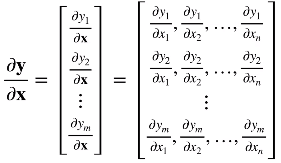
(3) Derivative of a vector with respect to a vector

The derivative of a vector with respect to a vector is a matrix:

3.2 Vector Chain Rule

Chain rule for scalars:

$y=f(u),u=g(x)$, so $\frac{\partial y}{\partial x}=\frac{\partial y}{\partial u}\frac{\partial u}{\partial x}$

Chain rule for vectors:

$\frac{\partial y}{\partial \textbf x}=\frac{\partial y}{\partial u}\frac{\partial u}{\partial \textbf x}$ (1,n) = (1, )(1, n)

$\frac{\partial y}{\partial \textbf x}=\frac{\partial y}{\partial \textbf u}\frac{\partial \textbf u}{\partial \textbf x}$ (1,n) = (1, k)(k, n)

$\frac{\partial \textbf y}{\partial \textbf x}=\frac{\partial \textbf y}{\partial \textbf u}\frac{\partial \textbf u}{\partial \textbf x}$ (m,n) = (m,k)(k.n)

3.3 Automatic Differentiation

Automatic differentiation computes the derivative of a function at a specified value.

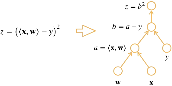
(1) Computation graphs

A computation graph reverse-knots code into operators and represents computation as an acyclic graph. It amounts to applying the chain rule during differentiation.

(2) Modes of automatic differentiation

Chain rule: $\frac{\partial y}{\partial x}=\frac{\partial y}{\partial u_n}\frac{\partial u_n}{\partial u_{n-1}}\cdots \frac{\partial u_2}{\partial u_1}\frac{\partial u_1}{\partial x}$

• Forward accumulation: $\frac{\partial y}{\partial x}=\frac{\partial y}{\partial u_n}(\frac{\partial u_n}{\partial u_{n-1}}(\cdots (\frac{\partial u_2}{\partial u_1}\frac{\partial u_1}{\partial x})))$

• Reverse propagation: $\frac{\partial y}{\partial x}=(((\frac{\partial y}{\partial u_n}\frac{\partial u_n}{\partial u_{n-1}})\cdots) \frac{\partial u_2}{\partial u_1})\frac{\partial u_1}{\partial x}$

In general, for input data we first run a forward pass to compute the result, then a backward pass to compute gradients. The forward pass saves all intermediate variables. When computing gradients, we already have the concrete values of abz, so we can substitute them directly to obtain derivatives—for example, dz/db=2b. Likewise, the derivatives of other operators can be obtained by direct substitution; according to the chain rule, the final gradient is the product of the derivatives of each operator.

(3) PyTorch implementation of automatic differentiation

Suppose we differentiate the function $\textbf y=2\textbf x^T \textbf x$ with respect to the column vector $\textbf x$

import torch

# 创建输入
x = torch.arange(4.0)

# 创建一个空间存储梯度值，执行后x.grad就可以存储梯度值，默认为none
x.requires_grad_(True)

# 计算y
y = 2 * torch.dot(x, x)

# 调用反向传播函数计算y关于x每个分量的梯度，结果将自动保存在x.grad中
y.backward()

# 默认情况下，pytorch会累计梯度，如果需要计算其他函数的梯度，需要先清除之前的值
x.grad.zero_()

Sometimes we need to move certain parameters outside the computation graph:

# 清空x.grad
x.grad.zero_()

# 定义y
y = x * x

# 将y从计算图中剔除，y的当前结果保存为u，则u=x*x是一个固定的值
u = y.detach()

# 此时u和x无关，u.backward()是0向量
# y仍然和x有关，y.backward()是2 * x

The steps above save the current value of y as u while leaving y unchanged. This kind of operation is used in deep learning.