[Deep Learning Notes 07] Convolutional Neural Network

I. Convolution Operations

As mentioned earlier, for a neural network such as face recognition, earlier layers mainly extract edges from the image, middle layers mainly detect parts such as eyes, nose, and mouth, and later layers mainly detect the full face.

1.1 How to Detect Edges

Different convolution kernels, also called filters, are commonly used to perform various types of edge detection.

(1) Vertical edges

Use the following convolution kernel for detection:

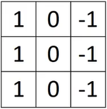
For example, for an image with vertical edges, applying this convolution kernel produces larger values at the edges and smaller values in regions where the image changes slowly.

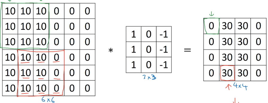
The convolution above can effectively determine where edges are in the image. If the convolution result is positive, the image changes from bright to dark from left to right; if negative, it changes from dark to bright from left to right.

(2) Horizontal edges

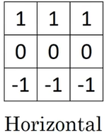
This convolution kernel can compute horizontal edges in the image. A positive value means brighter on top and darker on the bottom; the larger the value, the more pronounced the edge change.

(3) Other filters

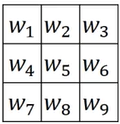
By defining the distribution of values in the convolution kernel, you can detect edges in different directions—not only horizontal and vertical, but also 45 or 75°.

You can also change the values in each row—for example, 1:2:1—to achieve more targeted detection.

1.2 Padding

(1) Problems with ordinary convolution

• Image shrinkage: For an (n, n) image, convolving with an (f, f) kernel yields an output of size (n-f+1, n-f+1), so each convolution reduces the image size.
• Loss of edge information: Corner pixels are processed by only one convolution window, and edge pixels tend to lose more information compared to central pixels.

(2) Solution

Before performing the convolution, pad the image border with an extra layer of pixels.

For example, if p layers of pixels are added around the image border, the output size after convolution is (n+2p-f+1, n+2p-f+1).

Typically, the side length of the convolution kernel is odd.

1.3 Convolution Stride

With an (f, f) convolution kernel applied to an (n, n) image, padding p, and stride s, the output dimensions are $(\frac{n+2p-f}{s}+1, \frac{n+2p-f}{s}+1)$

II. Three-Dimensional Convolution

2.1 Basics of Three-Dimensional Convolution

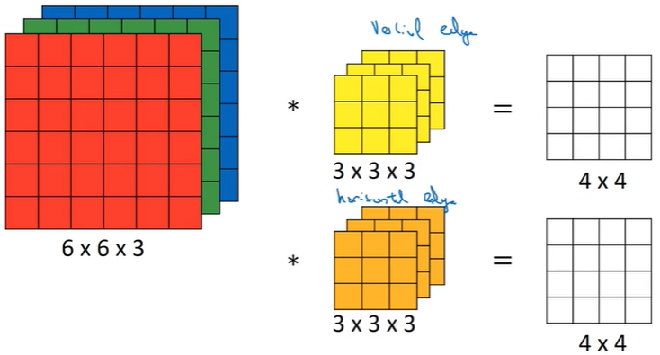
For example, an RGB image has dimensions (w, h, 3). To convolve it, the kernel must have dimensions (f, f, 3).

That is, the number of channels in the image and the convolution kernel must match.

After convolution, the output is an n-channel image of size (w-f+1, h-f+1, n), where n is the number of convolution kernels.

2.2 Three-Dimensional Convolution in Neural Networks

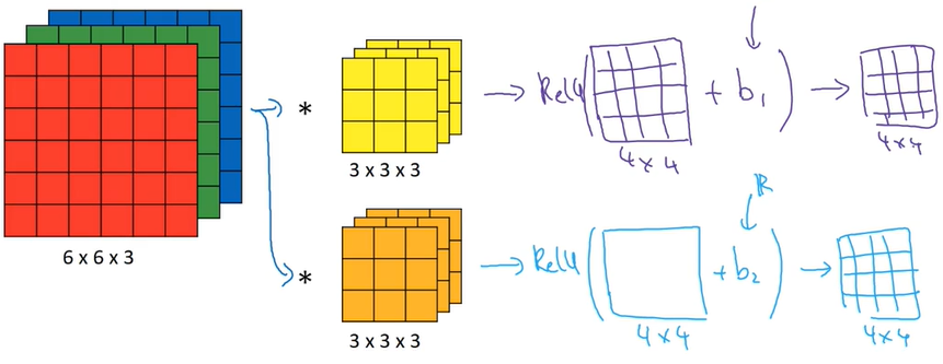
Applying three-dimensional convolution in neural networks is largely the same as the traditional approach.

In the traditional approach, $z^{[1]}=w^{[1]}a^{[0]}+b^{[1]}$, where $a^{[0]}$ is the input x and $a^{[1]}=g(z^{[1]})$.

For convolution, simply replace x with the input image and w with the convolution kernels, then add bias and a nonlinear activation function in the same way.

III. Pooling Layers

Pooling layers can reduce model size, speed up computation, and improve model robustness.

3.1 Max Pooling

For example, with a 4x4 input and 2x2 max pooling, the output divides the 4x4 input into 4 parts and fills a 2x2 output with the maximum value from each part. The output dimensions of max pooling are computed the same way as for convolution.

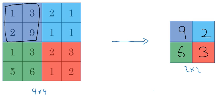
Max pooling keeps the largest value when a convolutional filter has extracted a feature; when no feature is extracted, the maximum remains small.

3.2 Average Pooling

Average pooling is similar to max pooling, but computes the average within each region. It is mainly used in very deep networks.

Currently, max pooling is more commonly used than average pooling.

3.3 Pooling Summary

The main pooling parameters are:

• f: pooling filter size
• s: compensation
• max or average pooling

Since pooling layers have no weights and only the hyperparameters above, convolution layers and pooling layers are generally counted together as one layer.

IV. Fully Connected Layers

At the end of a neural network, after multiple rounds of convolution and pooling, the final output often has small width and height but many channels. We then flatten it into a vector whose length equals the previous layer’s $w\times h\times c$. All parameters in that vector serve as inputs to the same number of units for conventional neural network computation—this is the fully connected layer.

V. Code Implementation

(1) Adding padding

def zero_pad(X, pad):
    """
    对数据集X的所有图像添加pad，padding被应用再一张图片的宽和高方向上。
    参数:
    X -- numpy数组，shape (m, n_H, n_W, n_C) 代表批量为m的图片
    pad -- 整数，图片边缘填充的pad大小
    Returns:
    X_pad -- 添加了以0填充的pad图片，shape (m, n_H + 2*pad, n_W + 2*pad, n_C)
    """

    X_pad = np.pad(X, ((0, 0), (pad, pad), (pad, pad), (0, 0)))

    return X_pad

(2) Single-step convolution (NumPy implementation)

def conv_single_step(a_slice_prev, W, b):
    """
    在上一层的一个切片用卷积核W进行卷积, 并添加偏差b
    
    参数:
    a_slice_prev -- 输入数据的切片，shape (f, f, n_C_prev)
    W -- 权重参数，以卷积核的形式体现，shape (f, f, n_C_prev)
    b -- 偏置参数，shape (1, 1, 1)

    返回值:
    Z -- 标量，滑动窗口(W, b)与输入切片x的卷积计算的结果
    """
    # a_slice 和 W 按元素相乘并添加偏置.
    S = np.multiply(W, a_slice_prev) + b
    # 求和
    Z = np.sum(S)
    
    return Z

(3) Three-dimensional convolution (NumPy implementation)

def conv_forward(A_prev, W, b, hparameters):
    """
    卷积前向计算
    
    参数:
    A_prev -- 上一层的激活输出，shape (m, n_H_prev, n_W_prev, n_C_prev)
    W -- 权重, shape (f, f, n_C_prev, n_C)
    b -- 偏置, shape (1, 1, 1, n_C)
    hparameters -- 包含 "stride" 和 "pad" 的字典
        
    返回值:
    Z -- 卷积输出，shape (m, n_H, n_W, n_C)
    cache -- 缓存，用于conv_backward()函数
    """
    
    # 获取 A_prev 的维度  
    m, n_H_prev, n_W_prev, n_C_prev = A_prev.shape

    # 获取 W 的维度
    f, _, n_C_prev, n_C = W.shape
    
    # 获取 hparameters 中的参数
    stride = hparameters["stride"]
    pad = hparameters["pad"]

    # 计算卷积输出的维度
    n_H = (n_H_prev - f + 2 * pad) // stride + 1
    n_W = (n_W_prev - f + 2 * pad) // stride + 1
    n_C = W.shape[3]
    
    # 零初始化卷积输出变量Z
    Z = np.zeros((m, n_H, n_W, n_C))
    
    # 调用函数，填充0创建 A_prev_pad 
    A_prev_pad = zero_pad(A_prev, pad)
    
    # 在训练样本的批量中循环
    for e in range(m):
        # 选择第e个填充样本
        A_prev_pad_e = A_prev_pad[e]
        # 在输出Z的竖直方向遍历
        for h in range(n_H):
            # 在输出Z的水平方向遍历
            for w in range(n_W):
                # 遍历所有通道，通道数为卷积核个数
                for c in range(n_C):
                    # Find the corners of the current "slice" (≈4 lines)
                    vert_start = h * stride
                    vert_end = vert_start + f
                    horiz_start = w * stride
                    horiz_end = horiz_start + pad
                    
                    # 确定被卷积区域
                    A_prev_pad_slice = A_prev_pad_e[vert_start:vert_end, horiz_start:horiz_end, :]
                    
                    # 使用卷积核W和偏置b进行卷积
                    Z[e, h, w, c] = np.sum(np.multiply(A_prev_pad_slice, W[:, :, :, c]) + b[:, :, :, c])

    # 确保输出维度正确
    assert(Z.shape == (m, n_H, n_W, n_C))
    
    # 将信息保存在cache中，用于反向传播
    cache = (A_prev, W, b, hparameters)
    
    return Z, cache

(4) Pooling

# GRADED FUNCTION: pool_forward

def pool_forward(A_prev, hparameters, mode = "max"):
    """
    前向传播的池化层
    
    参数:
    A_prev -- 输入数据，shape (m, n_H_prev, n_W_prev, n_C_prev)
    hparameters -- 包含 "f" 和 "stride" 的python字典
    mode -- 想要使用的池化模式, 定义为字符串 ("max" or "average")
    
    返回值:
    A -- 池化层输出，shape (m, n_H, n_W, n_C)
    cache -- 保存池化层的数据，用于反向传播
    """
    
    # 获取输入数据的维度
    (m, n_H_prev, n_W_prev, n_C_prev) = A_prev.shape
    
    # 从 "hparameters" 中获取超参数
    f = hparameters["f"]
    stride = hparameters["stride"]
    
    # 定义输出维度
    n_H = int(1 + (n_H_prev - f) / stride)
    n_W = int(1 + (n_W_prev - f) / stride)
    n_C = n_C_prev
    
    # 初始化输出矩阵A
    A = np.zeros((m, n_H, n_W, n_C))              
                
    # 在训练样本的批量中循环
    for e in range(m):
        # 在输出Z的竖直方向遍历
        for h in range(n_H):
            # 在输出Z的水平方向遍历
            for w in range(n_W):
                # 遍历所有通道
                for c in range(n_C):
                    # 找到当前要进行池化的区域
                    vert_start = h * stride
                    vert_end = vert_start + f
                    horiz_start = w * stride
                    horiz_end = horiz_start + f

                    # 使用上面的角坐标定义slice区域
                    A_prev_slice = A_prev[e, vert_start:vert_end, horiz_start:horiz_end, c]
                    
                    # 根据池化模式在slice进行计算，求最大值或平均值
                    if mode == "max":
                        A[e, h, w, c] = np.max(A_prev_slice)
                    elif mode == "average":
                        A[e, h, w, c] = np.mean(A_prev_slice)

    
    # 保存输入和超参数，用于反向传播
    cache = (A_prev, hparameters)
    
    # 确保输出维度正确
    assert(A.shape == (m, n_H, n_W, n_C))
    
    return A, cache