[Deep Learning Notes 06] Hyperparameter Tuning and Handling

I. Hyperparameter Values

Parameters that usually need to be handled include:

Parameter	Typical value range	Tuning importance
Learning rate $\alpha$	0.1	Most important
Momentum	0.9	Important
Optimization parameters $\beta_1,\beta_2,\epsilon$	$\beta_1=0.9,\beta_2=0.999,\epsilon=10^{-8}$	Usually left unchanged
Number of layers		General
Number of hidden units		Important
Learning rate decay		General
Mini-batch size		Important

How to tune and choose parameters:

1. First, randomly sample parameters over a wide range and evaluate the effect of those random points to identify which hyperparameter has the greatest impact. For real problems, it is hard to know in advance which hyperparameter matters more; testing them one by one often fails to reveal the parameter that actually needs tuning.
2. Use a coarse-to-fine strategy: find the parameter ranges that perform well in random testing, then zoom in on those ranges and sample more densely within them to search for the best hyperparameter choices.

How to sample random values effectively

For example, when searching for a learning rate $\alpha$, the possible range might be 0.0001-1. With ordinary uniform random sampling, about 90% of the values would fall in 0.1-1, and only 10% in 0.0001-0.1, whereas in practice the learning rate is more likely to lie in the latter range.

To address this, you can sample on a logarithmic axis. Random sampling on a log scale greatly increases the number of values taken in 0.0001-0.1.

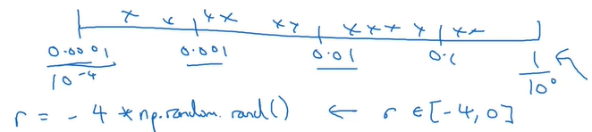
As another example, when searching for a momentum value $\beta$, the range might be 0.9-0.999, but the actual value will definitely be closer to 0.9. You can apply the same method to $1-\beta$ in [0.001, 0.1] to sample $\beta$ indirectly.

Why use a nonlinear axis for sampling? Because hyperparameters have different sensitivity to the result in different ranges. Take momentum $\beta$ as an example: at 0.9, changing it to 0.9001 affects the result much more than at 0.999, changing it to 0.9991. So we need more samples in the high-sensitivity range, which is why nonlinear-axis sampling is used.

II. Batch-Normalization (BN)

2.1 Basic idea of BN

In logistic regression, we used normalization (computing the mean and variance), which improved the training samples and sped up gradient descent.

In deep networks, however, the data used for gradient descent in the next layer are the output of the previous layer. In practice, the previous layer’s data are normalized before activation, then activated and passed to the next layer.

In a neural network, suppose there are hidden unit values $z^{(1)}\dots z^{(m)}$. Compute:

$\mu=\frac{1}{m}\sum_i z^{(i)}$ $\sigma^2=\frac{1}{m}\sum_i(z_i-\mu)^2$ $Z^{(i)}_{norm}=\frac{z^{(i)}-\mu}{\sqrt{\sigma^2+\epsilon}}$

This standardizes the output z of each layer. The result has mean 0 and variance 1. Although we want to use regularization to standardize the data and speed up gradient descent, we do not want every layer to follow exactly the same mean and variance, so we use the following variant:

$\widetilde z^{(i)}=\gamma z_{norm}^{(i)}+\beta$

Here $\gamma,\beta$ are new hyperparameters that set the mean and variance of the output z.

2.2 Why BN works

BN allows the weights to change more slowly than the network, or in deeper layers.

For a given layer, its input is the output of the previous layer. As parameters are updated, that previous output changes continuously, so the current layer always trains on inputs from a shifting distribution.

After using BN, the previous layer’s data can be normalized to the same distribution, making the previous layer’s output data more stable, thereby ensuring later layers have a better foundation.

In short, BN weakens the link between earlier-layer parameters and later-layer parameters, so each layer can learn somewhat independently of the rest of the network, which helps speed up learning for the whole network.

III. Softmax

3.1 Softmax notation

The classification methods mentioned earlier are for binary classification, whereas softmax regression applies to multi-class classification. We often use C to denote the number of input classes, which also equals the number of output units.

In use, simply replace the final layer’s activation function with softmax.

Suppose the last layer of the network is $l$. The softmax layer then computes as follows:

Compute the linear part: $z^{[l]}=w^{[l]}a^{[l-1]}+b^{[l]}$

Compute temporary variables: $t=e^{z^{[L]}}$

Compute the output—the probability of each class: $a^{[l]}=\frac{t_i}{\sum t_i}$

If $z^{[l]}$ is a (4,1) vector, then $t,a^{[l]}$ are both (4,1), and the four values in $a^{[l]}$ are the probabilities of the four classes.

3.2 Training a softmax network

(1) Loss function

Because the softmax output has the same dimension as the number of classes, a new loss function is needed.

$l(\hat y,y)=-\sum_{j=1}y_jlog\hat y_j$

To keep the loss small, we need $log\hat y_j$ to be as large as possible—that is, the corresponding probability should be as large as possible.

(2) Gradient descent

The key step is differentiating the softmax layer:

$dz^{[l]}=\hat y-y$