[Deep Learning Notes 08] Classic Neural Networks

I. Object Localization

1.1 Basic Idea

Object localization developed from image classification, while object detection is built on object localization.

For an image, we can use a convolutional neural network and the softmax function to classify it as, for example, a person, car, or bicycle.

If we want to locate an object in the image, we can have the softmax function output several additional numbers, such as 4 numbers describing the position of the bounding box (bx, by, w, h). The training set would then include not only image classification data but also the coordinates of the bounding boxes in the images.

1.2 Label Definition

Based on the idea above, we can define the image label as follows:

$y = [P_c, b_x, b_y, b_w, b_h, c_1, c_2, c_3]^T$

where

• $P_c$: indicates whether an object is present in the image (distinguishing objects from the background)
• $b_x, b_y, b_w, b_h$: the center coordinates, width, and height of the bounding box
• $c_1, c_2, c_3$: the probabilities that the object in the image belongs to each of three classes

1.3 Loss Function Design

For the label defined above, if we use a squared-loss strategy, the loss function is defined as follows:

If $y_1=1$, meaning that the image contains a target object:

$l(\hat y, y)=(\hat y_1-y_1)^2+(\hat y_2-y_2)^2+\dots+(\hat y_8-y_8)^2$

(Because the label contains 8 elements, they range from $y_1$ to $y_8$.)

If $y_1=0$, meaning that the image does not contain a target object:

$l(\hat y, y)=(\hat y_1-y_1)^2$

II. Landmark Detection

Above, we introduced how to output bounding-box coordinates by adding the 4 parameters $b_x, b_y, b_w, b_h$ to the label.

Landmark detection works on a similar principle.

Suppose that, for some reason, we want to obtain the coordinates of the four corners of a person’s eyes in an image. We can simply add them to the label, annotate the eye-corner coordinates of each person in the training images in advance, and then train a neural network.

$y = [P_c, l_{1x}, l_{1y}, l_{2x}, l_{2y}, \dots, l_{4x}, l_{4y}]^T$

where

• $P_c$: indicates whether a face is present in the image (image classification)
• $l_{1x}, l_{1y}, \dots, l_{4x}, l_{4y}$: the xy coordinates of the four eye corners

This follows the same principle as obtaining bounding boxes and classifying images.

If we want to go further and capture facial expressions, we can define multiple landmarks on a face, annotate the face in each image, and then use a neural network to perform regression.

In this way, landmark detection can be implemented.

III. Object Detection

Object detection is based on image classification.

3.1 Sliding-Window Method

Take car detection as an example:

For the training set, we can use images in which a car occupies the entire area as training images. These can be obtained by cropping the areas occupied by cars from other photos.

For a given image, we select a small window within the image and feed the image inside that window into a neural network to determine whether it contains a car. We then move the small window to the next position and continue detecting. After traversing the entire image, we adjust the window size and traverse it again.

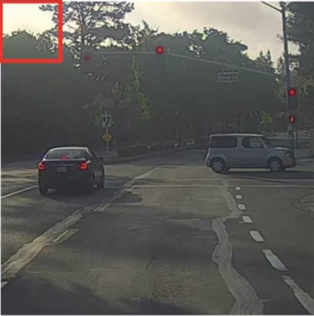
This algorithm is generally called the sliding-window method.

Its advantage is that the algorithm is simple to design, but it also has the clear disadvantage of requiring too much computation. The window size and stride must also be chosen appropriately; otherwise, objects in the image cannot be located accurately.

3.2 Obtaining More Precise Bounding Boxes

Existing problems with the sliding-window method:

• If the stride is large, the selected window often cannot fully cover the target object. If the stride is small, the computational cost becomes excessive.
• The target object is sometimes not a regular square, so a square sliding window does not produce a sufficiently precise bounding box.

Solution:

1. Use an object localization algorithm to divide the image into 9 grid cells, perform object localization on each grid cell, and train using a label similar to $y = [P_c, b_x, b_y, b_w, b_h, c_1, c_2, c_3]^T$.
2. Each grid cell will then produce an output, such as $y = [1, b_x, b_y, b_w, b_h, 0, 1, 0]^T$. Taken together, the output dimensions are 3x3x8. Here, 3x3 is the number of grid cells, and 8 is the number of output parameters.

Compared with the sliding-window method, which outputs the window with the greatest coverage as the bounding box, this method instead regresses the bounding box as four parameters.

Advantages:

• Because many computational steps are shared when different grid cells are processed using convolutions, computational efficiency is greatly improved.
• Because it is implemented using convolutions, it is very fast and can achieve real-time recognition.

3.3 NMS (Non-Max Suppression)

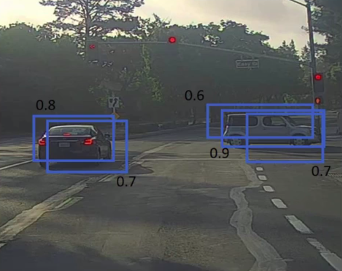
Problem: The algorithm may identify the same object multiple times. We need to take some measure to ensure that the algorithm detects each object only once.

Solution:

Among the output results, find the one with the highest identification probability, such as 0.9 in the figure, and suppress the other boxes with a large intersection over union with this box. We consider the box with a probability of 0.9 to have marked an object.

Then find the box with the highest probability among all the remaining boxes, such as 0.8 in the figure, and suppress the other boxes with a large intersection over union with this box to obtain the prediction results.

Intersection over union $IOU=\frac{交集区域}{并集区域}$

Implementation process:

• Divide the image into nxn grid cells and make a prediction for each one, obtaining parameters including the probability that an object is present and the position and size of the bounding box.
• Delete all bounding boxes whose object-presence probability is less than 0.6.
• For the remaining bounding boxes:
  • Select the bounding box with the highest probability as an output, consider it to have marked an object, and delete bounding boxes whose overlap with it exceeds 50%.
  • From the remaining bounding boxes, again find the one with the highest probability as an output, consider it to have marked another object, and delete bounding boxes whose overlap with it exceeds 50%.
  • Repeat the process.