[Deep Learning Notes 04] Elements for Improving Training Performance and Speed

I. Training Set, Validation Set, and Test Set

For input data, we usually split it into several parts: training set, cross-validation set, and test set.

In the earlier era of machine learning with small datasets, people typically split all data into 60% training, 20% validation, and 20% test. That was widely considered a reasonable approach at the time.

In the big-data era, the validation and test portions become smaller. For example, with one million data points, we might use only 10,000 for validation and 10,000 for testing—that is, 98% training, 1% validation, and 1% test.

When choosing data splits, make sure the validation set and test set come from the same distribution.

II. Bias and Variance

When bias is too high, the fitted curve may differ greatly from the actual values—that is underfitting.

When variance is too high, the fitted curve becomes overly complex—that is overfitting.

When the training error is much lower than the validation error, we have overfit the training set and failed to make full use of the cross-validation set. This is the high-variance case.

When both the training error and validation error are high, the training data are not fit well—underfitting, or the high-bias case.

Training set error rate

III. Machine Learning Basics

First we need to evaluate the algorithm’s bias. If bias is high, puzzled we can try a new network, add more hidden layers, or spend more time training the algorithm and scale up the network—these methods may work, or they may not.

Then evaluate the algorithm’s variance. If variance is high, the best fix is to add more data; we can also use regularization to reduce overfitting.

When we find an algorithm with low bias and low variance, we have succeeded at machine learning.

Note that bias and variance are two different problems and require different solutions.

IV. Regularization

4.1 How to Implement Regularization

When a neural network overfits—that is, when variance is high—we usually think of regularization. (Another common approach is to increase the amount of data.)

Add regularization to the loss function $J(w,b)$:

$J(w,b)=\frac{1}{m}\sum^m_{i=1}l(\hat y^{(i)},y^{(i)})+\frac{\lambda}{2m}||w||_2^2$

where $\frac{\lambda}{2m}||w||^2_2$ is the regularization term, also called $L_2$ regularization (because it uses $||w||^2$). This is also the most widely used form of regularization. The $L_1$ regularization term is $\frac{\lambda}{2m}\sum^{n_x}_{j=1}|w_j|$.

$\lambda$ is the regularization parameter. We need to tune it using the validation set—try various datasets to adjust the parameter—so $\lambda$ is a hyperparameter.

In a neural network:

$J(w^{[1]}, b^{[1]}\dots w^{[L]}, b^{[L]})=\frac{1}{m} \sum^n_{i=1}l(\hat y, y)+\frac{\lambda}{2m}\sum^L_{l=1}||w^{[l]}||^2_F$

where $||w^{[l]}||^2_F=\sum^{n^{[l-1]}}_{i=1}\sum^{n^{l}}_{j=1}(w_{ij}^{[l]})^2$, called the Frobenius norm, is the sum of squares of all elements in the matrix.

When computing gradients we compute $\frac{\partial J}{\partial w}$, so the resulting gradient includes an extra regularization term on top of the original one:

$dw^{[l]}=(backprop)+\frac{\lambda}{m}w^{[l]}$

So during parameter updates, a regularization term is also applied:

$w^{[l]}=w^{[l]}-\alpha[(backprop)+\frac{\lambda}{m}w^{[l]}]$

This is equivalent to shrinking the step size of parameter updates, so $L_2$ regularization is also called weight decay.

4.2 Why Regularization Can Reduce Overfitting

After adding regularization, we can avoid weight matrices becoming too large.

Intuitively, if the regularization parameter $\lambda$ is set large enough, the weight matrix will be pushed toward values close to 0, which removes much of the influence of those hidden units. The whole network then resembles a high-bias situation with many hidden layers but only one hidden unit per layer.

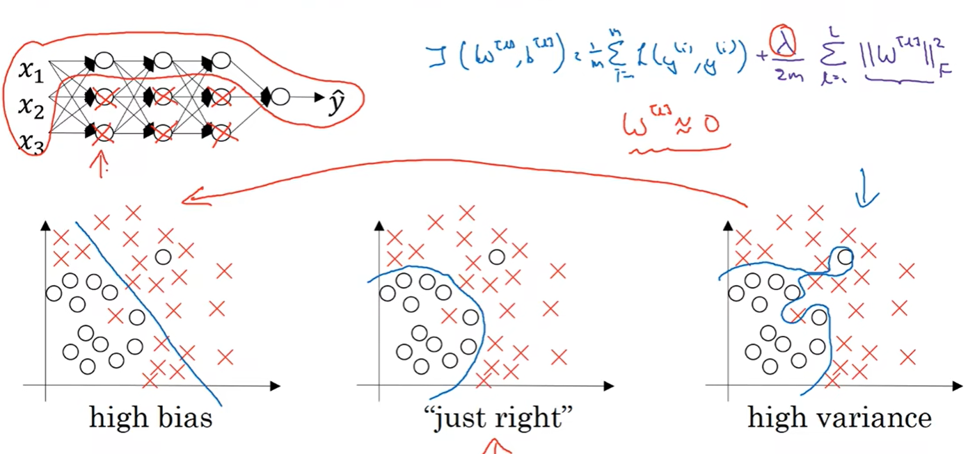
On the other hand, when the weight matrix W is small, $Z=Wa+b$ is also small. For activation functions like tanh, $g(z)$ falls in the nearly linear region near the two sides of the y-axis, which simplifies the model and makes overfitting less likely.

4.3 Dropout Regularization

Dropout goes through each layer of the network and assigns a probability of dropping or keeping each neuron. After that setup, some nodes are dropped in each layer. The pruned model is then trained with backpropagation; for all samples we set these probabilities randomly.

(1) How to Implement Dropout Regularization

The most common method is inverted dropout.

Take a three-layer network as an example. First define the vector d3=np.random.rand(a3.shape[0], a3.shape[1])—that is, d3 has the same latitude as a3.

Compare d3<keep.prob, which represents the probability of keeping hidden units. Set elements in d3 that are less than keep.prob to 1, and those greater than keep.prob to 0.

Then filter out all elements in d3 that equal zero: a3=np.multiply(a3,d3).

Scale a3 outward: a3/=keep.prob. This is mainly to keep the expected value of Z in $Z=Wa+b$ unchanged. Because 80% of the elements in a are dropped, the remaining elements are scaled up by 1/0.8 so the expectation of Z stays the same.

(2) How to Understand Dropout Regularization

For each neuron, its input features (nodes from the previous layer) may be dropped at any time, so it cannot rely on any single feature and will not place too much weight on any one input. It therefore treats all inputs equally.

Moreover, different layers can use different keep.prob values. For layers that may overfit, keep.prob can be set lower than in other layers.

Dropout is typically applied in computer vision; it is not used as widely in other fields.

Because nodes are immediately dropped each iteration, it is hard to evaluate J; J will not decrease monotonically. Usually we turn off dropout regularization first, then debug until J decreases monotonically, at turn it on.

4.4 Other Regularization Methods

(1) Data Augmentation

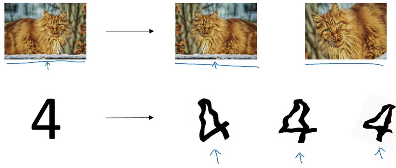
For image classification, if we want to expand the dataset we can flip, rotate, scale and crop images, then add them to the dataset. Although this is less effective than collecting new data, it still helps reduce overfitting.

(2) Early Stopping

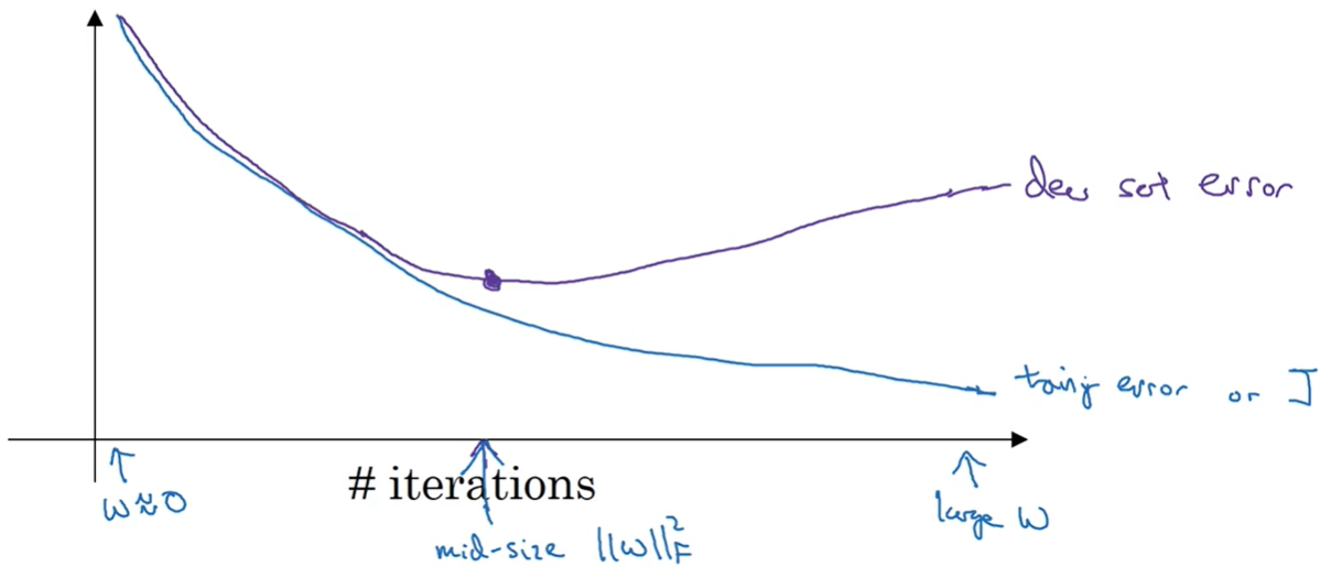
When running gradient descent, we can plot the loss curve (usually monotonically decreasing) and also plot the error on the validation set. We usually find validation-machine error falls first and then rises; we can stop at the point where validation set error is smallest.

V. Normalization

Suppose we have a training set with two inputs. Normalizing the inputs has two steps:

(1) Zero-mean normalization

$\mu=\frac{1}{m}\sum^m_{i=1}x^{(i)}$ $x=x-\mu$

(2) Normalization

$\sigma^2=\frac{1}{m}\sum^m_{i=1}x^{(i)^2}$ $x/=\sigma$

After this, x1 and x2 form a dataset centered at 0 with variance 1.

(3) Why Standardize

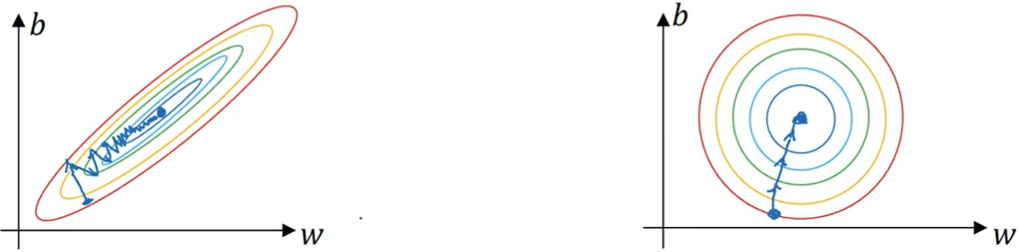
If the two input features differ greatly in scale, the values in the weight matrix W1 and W2 will also differ greatly. That makes the gradient surface of the loss function very uneven, and the learning rate must be set very small to reach the optimum.

By contrast, after normalization, gradient descent can reach the optimum well from any starting point.

VI. Vanishing and Exploding Gradients

For a very deep neural network, the prediction $\hat y$ might look like this:

$\hat y=w^{[l]}+w^{[l-1]}+\dots+w^{[3]}+w^{[2]}+w^{[1]}$

If each layer’s w is greater than 1, then $\hat y$ and gradients such as $dw$ can grow explosively. If each layer’s w is less than 1, then $\hat y$ shrinks exponentially.

VII. Weight Initialization

For a given node, if it has many input features—for example:

$z=w_1x_1+w_2x_2+\dots+w_nx_n$

then as the number of input features n grows, each weight $w_i$ should be smaller.

A common approach is to scale each $w_i$ down by a factor of $\frac{1}{n}$. In practice we use:

$W^{[l]}=np.random.randn(shape)*np.sqrt(\frac{2}{n^{[l-1]}})$

For the ReLU activation function, use $np.sqrt(\frac{2}{n^{[l-1]}})$ on the right.

For the tanh activation function, use $np.sqrt(\frac{1}{n^{[l-1]}})$, or $np.sqrt(\frac{2}{n^{[l-1]}+n^{[l]}})$, on the right.

The 1 or 2 in the numerator can also be tuned as a hyperparameter, though it does not matter much.

VIII. Gradient Checking

Note that gradient checking is only for debugging. Do not enable it during actual training, because it is too slow.

Suppose the network has parameters $W^{[1]},b^{[1]}\dots W^{[l]},b^{[l]}$.

First convert all parameter matrices into vectors and concatenate them into one large vector $\theta$.

Thus $J(W^{[1]},b^{[1]}\dots W^{[l]},b^{[l]})=J(\theta)$.

Likewise obtain one large gradient vector $d\theta$.

(1) Compute the approximate gradient

$d\theta_{approx}[i]=\frac{J(\theta_1,\theta_2,\dots,\theta_i+\epsilon,\dots)-J(\theta_1,\theta_2,\dots,\theta_i-\epsilon,\dots)}{2\epsilon}$

Here $\epsilon$ is usually set to $10^{-7}$.

(2) Measure the distance between the approximate gradient and the computed gradient

We usually use the Euclidean distance $\frac{||d\theta_{approx}-d\theta||_2}{||d\theta_{approx}||+||d\theta||}$.

If the distance is around $10^{-7}$, things look fine. If it is too large—for example, $10^{-5}$—something may be wrong somewhere. You can compute it for each i individually to see which step has the problem.