[Deep Learning Notes 05] Common Optimization Algorithms in Deep Learning

Mini-batch Gradient Descent

(1) Why mini-batch is needed

We know that in neural networks we often use vectorization to process all m examples more quickly.

However, for an extremely large number of examples—for instance, a dataset with 1 million samples—vectorization means creating a huge matrix with 1 million columns and processing the entire dataset before taking another gradient-descent step. This approach is called batch gradient descent.

To address this problem, we can split the training set into smaller sub-training sets called mini-batches—for example, taking 1,000 samples for training each time, then taking another 1,000 samples for the next round of training.

(2) How to understand mini-batch

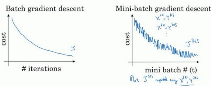
When using mini-batch gradient descent, each iteration processes $X^{\{t\}}$ and $y^{\{t\}}$, so the cost curve looks different depending on which subset is used. Because the weights and biases are optimized gradually over training, the overall cost still trends downward with oscillations.

(3) Hyperparameter: batch_size

One hyperparameter used when setting up mini-batches is the batch size. If the training set has size m:

• batch_size=m: each mini-batch is the entire training set, which is batch gradient descent. This case has relatively lower noise and larger steps, and you can continue searching for the minimum afterward.
• batch_size=1: this is called gradient descent; each example is its own mini-batch. In most cases this method moves toward the minimum, but sometimes moves away from it, with a lot of noise, and this method will never bracelet—it keeps oscillating near the minimum.

In practice, the mini-batch size is usually chosen between these two extremes, i.e., 1<batch_size<m. If the number of samples is small, there is no need to partition subsets; just use batch gradient descent directly. For larger datasets, batch_size is generally chosen between 64 and 512, depending on available memory.

(4) Implementation

def random_mini_batches(X, Y, mini_batch_size = 64, seed = 0):
    """
    从(X, Y)创建随机的mini-batch
    
    参数:
    X -- 输入数据, shape (input size, number of examples)
    Y -- 真值向量, shape (1, number of examples)
    mini_batch_size -- mini-batches的大小，整形
    
    返回值:
    mini_batches -- 同步的列表 (mini_batch_X, mini_batch_Y)
    """
    
    np.random.seed(seed)
    m = X.shape[1]                  # 训练样本的数量
    mini_batches = []
        
    # Step 1: 打乱 (X, Y)
    permutation = list(np.random.permutation(m))
    shuffled_X = X[:, permutation]
    shuffled_Y = Y[:, permutation].reshape((1,m))

    # Step 2: 分区 (shuffled_X, shuffled_Y). 
    num_complete_minibatches = math.floor(m/mini_batch_size) # 以mini_batch_size为大小的分区的数量
    for k in range(0, num_complete_minibatches):
        mini_batch_X = shuffled_X[:, k*mini_batch_size : (k+1)*mini_batch_size]
        mini_batch_Y = shuffled_Y[:, k*mini_batch_size : (k+1)*mini_batch_size]
        mini_batch = (mini_batch_X, mini_batch_Y)
        mini_batches.append(mini_batch)
    
    # 处理剩余的样本（少于mini_batch_size的样本）
    if m % mini_batch_size != 0:
        mini_batch_X = shuffled_X[:, num_complete_minibatches*mini_batch_size : m]
        mini_batch_Y = shuffled_Y[:, num_complete_minibatches*mini_batch_size : m]
        mini_batch = (mini_batch_X, mini_batch_Y)
        mini_batches.append(mini_batch)
    
    return mini_batches

Momentum Gradient Descent

2.1 Exponentially Weighted Average

(1) What is an exponentially weighted average

An exponentially weighted average can fit a noisy, oscillating curve into a smooth one.

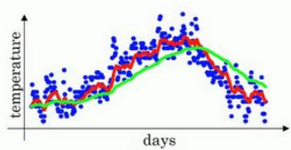
Its mathematical expression is:

$V_t=\beta V_{t-1}+(1-\beta)\theta_t$

(2) How to understand the exponentially weighted average

Take $\beta=0.9$ as an example. We can write:

$V_{100}=0.9V_{99}+0.1\theta_{100}$ $V_{99}=0.9V_{98}+0.1\theta_{99}$ $V_{98}=0.9V_{97}+0.1\theta_{98}$

Substituting the last two equations into the first gives:

$V_{100}=0.9V_{99}+0.1\theta_{100}$ $=0.1\theta_{100}+0.9(0.9V_{98}+0.1\theta_{99})$ $=0.1\theta_{100}+0.9(0.1\theta_{99}+0.9(0.9V_{97}+0.1\theta_{98}))$ $=0.1\theta_{100}+0.1\times 0.9\theta_{99}+0.1\times 0.9^2\theta_{98}++0.1\times 0.9^3\theta_{97}+\dots$

We can see that this is a weighted sum and average of $\theta$. For $V_{100}$, it is determined by the previous 99 data points; data closer to 100 receive larger weights, and data farther away receive smaller weights—the weights decay exponentially.

(3) Hyperparameter: $\beta$

In the formula $V_t=\beta V_{t-1}+(1-\beta)\theta_t$, a larger $\beta$ means slower weight decay during weighting, so it can be viewed as averaging over more data points. A smaller $\beta$ means faster weight decay during weighting, so it can be viewed as averaging over only the most recent few data points.

The advantage of the exponentially weighted average formula is that it uses very little memory: you only store the previous value, compute the latest data point, and overwrite it repeatedly, without reading in all data to fit the curve.

2.2 Momentum Gradient Descent

The basic idea is to compute a weighted average of the gradients and use that average to update the weights.

For example, when optimizing a cost function, gradient descent often oscillates up and down before reaching the minimum. These oscillations slow gradient descent and prevent using a larger learning rate, because if the learning rate is too large, the result may go outside the valid range of the function.

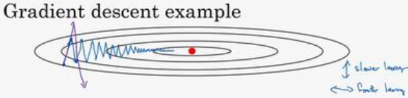
In summary, we want learning to proceed more slowly in the b direction to reduce unnecessary oscillation, and faster in the W direction to approach the minimum quickly.

Therefore, one workable approach is momentum gradient descent. At each iteration, compute the partial derivatives dW and db, then compute $V_{dW}=\beta V_{dW}+(1-\beta)dW$ and likewise $V_{db}=\beta V_{db}+(1-\beta)db$, and assign the computed values back to dW and db. What is the benefit of doing this?

Similar to the figure above, through weighted averaging, the oscillating gradient values dW and db become smoothly varying gradients. In the b direction, positive and negative values cancel out, reducing oscillation in dW; in the W direction, because all partial derivatives point the same way, movement in W becomes faster.

You can think of the cost function as a bowl-shaped surface and gradient descent as rolling a ball down the edge of the bowl. The $(1-\beta)dW$ and $(1-\beta)db$ terms provide acceleration at each moment, while $\beta v_{dW}$ and $\beta v_{db}$ are the instantaneous velocity from the previous moment. So the ball rolls faster and faster, and because $\beta$ is less than 1, it behaves somewhat like friction, so the ball does not accelerate without bound.

The momentum gradient descent procedure is therefore:

$V_{dW}=\beta V_{dW}+(1-\beta)dW$ $V_{db}=\beta V_{db}+(1-\beta)db$ $W=W-\alpha v_{dW}$ $b=b-\alpha v_{db}$

This process has two hyperparameters: momentum $\beta$ and learning rate $\alpha$

2.3 Implementation

def update_parameters_with_momentum(parameters, grads, v, beta, learning_rate):
    """
    使用动量更新参数
    
    参数:
    parameters -- 包含所有参数的python字典:
                    parameters['W' + str(l)] = Wl
                    parameters['b' + str(l)] = bl
    grads -- 包含所有参数的梯度的python字典:
                    grads['dW' + str(l)] = dWl
                    grads['db' + str(l)] = dbl
    v -- 包含当前速度的python字典:
                    v['dW' + str(l)] = ...
                    v['db' + str(l)] = ...
    beta -- 动量超参数，标量
    learning_rate -- 学习率，标量
    
    返回值:
    parameters -- 包含所有更新后的参数的python字典
    v -- 包含所有更新后的速度的python字典
    """

    L = len(parameters) // 2 # 神经网络的层数
    
    # 每个参数的Momentum更新
    for l in range(L):
        # 计算速度
        v['dW'+str(l+1)] = beta * v['dW'+str(l+1)] + (1 - beta) * grads['dW'+str(l+1)]
        v['db'+str(l+1)] = beta * v['db'+str(l+1)] + (1 - beta) * grads['db'+str(l+1)]
        # 更新参数
        parameters['W'+str(l+1)] -= learning_rate * v['dW'+str(l+1)]
        parameters['b'+str(l+1)] -= learning_rate * v['db'+str(l+1)]
        
    return parameters, v

RMSprop

RMSprop stands for root mean square prop and can also accelerate gradient descent.

The mathematical form is:

$S_{dW}=\beta S_{dW}+(1-\beta)dW^2$ $S_{dW}=\beta S_{dW}+(1-\beta)dW^2$

The parameter update is:

$W=W-\alpha \frac{dW}{\sqrt{S_{dW}}}$ $b=b-\alpha \frac{db}{\sqrt{S_{db}}}$

The idea is as follows:

We want fast learning while reducing oscillation. So we introduce $S_{dW}$ and $S_{db}$. We want $S_{dW}$ to be small, so we divide by a smaller number; we want $S_{db}$ to be large, so we divide by a larger number—this reduces oscillation along b. Moreover, among these partial derivatives, because the slope in the b direction is greater than in the W direction, db is larger and dW is smaller; dividing $S_{dW}$ by a smaller number means dW, and dividing $S_{db}$ by a smaller number means db—hence the formulas above.

Adam

Adam stands for Adaptive Moment Estimation. It combines momentum gradient descent and RMSprop.

The steps are:

$V_{dW}=\beta_1 v_{dW}+(1-\beta_1)dW$ $V_{db}=\beta_1 v_{db}+(1-\beta_1)db$ $S_{dW}=\beta_2 S_{dW}+(1-\beta_2)dW^2$ $S_{dW}=\beta_2 S_{dW}+(1-\beta_2)dW^2$

$W=W-\alpha \frac{V_{dW}}{\sqrt{S_{dW}}+\epsilon}$ $b=b-\alpha \frac{V+{db}}{\sqrt{S_{db}}+\epsilon}$

$\epsilon$ is commonly set to $10^{-8}$ to avoid division by 0—a small value added for that purpose.

This algorithm combines Momentum and RMSprop and has been shown to work well across different neural networks.

This algorithm involves several hyperparameters

• $\alpha$: learning rate
• $\beta_1$: the Momentum-related term; the commonly used default is 0.9
• $\beta_2$: the Adam-related term; the commonly used default is 0.99
• $\epsilon$: commonly $10^{-8}$; this parameter has little effect on the algorithm

Implementation

def update_parameters_with_adam(parameters, grads, v, s, t, learning_rate = 0.01,
                                beta1 = 0.9, beta2 = 0.999,  epsilon = 1e-8):
    """
    使用Adam进行参数更新
    
    参数:
    parameters -- 包含所有参数的python字典
                    parameters['W' + str(l)] = Wl
                    parameters['b' + str(l)] = bl
    grads -- 包含所有参数梯度的python字典
                    grads['dW' + str(l)] = dWl
                    grads['db' + str(l)] = dbl
    v -- Adam变量, 梯度一次项的移动的平均值, python字典
    s -- Adam变量, 梯度平方项的移动的平均值, python字典
    learning_rate -- 学习率，标量
    beta1 -- 第一种动量优化Momentum的指数衰减超参数
    beta2 -- 第二种动量优化RMSprop的指数衰减超参数
    epsilon -- 放置Adam参数更新过程中可能出现的0除现象

    返回值:
    parameters -- 包含所有更新后参数的字典
    v -- Adam变量, 梯度一次项的移动的平均值, python字典
    s -- Adam变量, 梯度平方项的移动的平均值, python字典
    """
    
    L = len(parameters) // 2                 # 神经网络的层数
    v_corrected = {}                         # 初始化第一种动量优化，字典
    s_corrected = {}                         # 初始化第二种动量优化，字典
    
    # 使用Adam方法更新所有参数
    for l in range(L):
        # 移动梯度的平均值. 输入: "v, grads, beta1". 输出: "v".
        v['dW'+str(l+1)] = beta1 * v['dW'+str(l+1)] + (1 - beta1) * grads['dW'+str(l+1)]
        v['db'+str(l+1)] = beta1 * v['db'+str(l+1)] + (1 - beta1) * grads['db'+str(l+1)]

        # 计算第一种动量优化的偏差矫正项. 输入: "v, beta1, t". 输出: "v_corrected".
        v_corrected['dW'+str(l+1)] = v['dW'+str(l+1)] / (1 - beta1 ** t)
        v_corrected['db'+str(l+1)] = v['db'+str(l+1)] / (1 - beta1 ** t)

        # 移动平方梯度的平均值. 输入: "s, grads, beta2". 输出: "s".
        s['dW'+str(l+1)] = beta2 * s['dW'+str(l+1)] + (1 - beta2) * (grads['dW'+str(l+1)] ** 2)
        s['db'+str(l+1)] = beta2 * s['db'+str(l+1)] + (1 - beta2) * (grads['db'+str(l+1)] ** 2)

        # 计算第二种动量优化的偏差矫正项. 输入: "s, beta2, t". 输出: "s_corrected".
        s_corrected['dW'+str(l+1)] = s['dW'+str(l+1)] / (1 - beta2 ** t)
        s_corrected['db'+str(l+1)] = s['db'+str(l+1)] / (1 - beta2 ** t)

        # 更新参数. 输入: "parameters, learning_rate, v_corrected, s_corrected, epsilon". 输出: "parameters".
        parameters['W' + str(l + 1)] -= learning_rate * v_corrected['dW' + str(l + 1)] / (np.sqrt(s_corrected['dW'+str(l+1)]) + epsilon)
        parameters['b' + str(l + 1)] -= learning_rate * v_corrected['db' + str(l + 1)] / (np.sqrt(s_corrected['db'+str(l+1)]) + epsilon)

    return parameters, v, s

Learning Rate Decay

During gradient descent, the process oscillates around the minimum but does not converge exactly. To keep the algorithm efficient, you can set a larger learning rate early on so learning is relatively fast and gradient descent proceeds quickly. Near the minimum, reduce the learning rate—take smaller steps—and gradually approach the minimum.

One approach is to decrease the learning rate slightly each time you pass through the entire dataset.

(1) The most commonly used decay formula

$\alpha=\frac{1}{1+decay\_rate\times epoch\_num}$

Here decay_rate is the decay rate and epoch_num is the iteration count. As epoch_num increases, the learning rate $\alpha$ gradually decreases.

(2) Exponential decay

$\alpha=0.95^{epoch\_num}\cdot\alpha_0$

(3) Inverse decay

$\alpha=\frac{k}{\sqrt{epoch\_num}}\cdot a_0$