Contents
- I. Introduction to Deep Learning
- 1.1 Neural Networks
- 1.2 Supervised Learning
- 1.3 About Deep Learning
- II. Fundamentals of Neural Network Programming
- 2.1 Notation
- 2.2 Binary Classification—The Logistic Regression Method
- 2.3 Gradient Descent
- 2.4 Computation Graphs
- 2.5 Vectorization
- 2.6 About numpy and Common Functions
I. Introduction to Deep Learning
1.1 Neural Networks
The activation function ReLU (basic rectified unit, Rectified linear unit) starts at zero and then rises along a straight line.
Every unit in a neural network may be a ReLU or another nonlinear unit.
1.2 Supervised Learning
(1) Application areas of deep learning
In supervised learning, X is first provided as input, and then a function is learned that maps the input to output Y.
Deep learning now plays an important role in fields such as online advertising, image processing, speech recognition, machine translation, and autonomous driving. However, for each application, we must choose x and y appropriately to solve the specific problem.
(2) Some commonly used architectures
Price prediction: general-purpose standard neural network (Standard NN) Image processing: convolutional neural network, CNN (Convolutional NN) Sequence processing, such as audio: recurrent neural network, RNN (Recurrent NN) Language processing uses more complex RNNs Autonomous driving uses images and radar, so it employs more complex hybrid neural network architectures
(3) Structured and unstructured data
Structured data is data in databases. For example, price prediction uses standard databases, while advertising uses databases containing user information, advertising information, and so on.
Unstructured data includes speech, images, videos, and text. Compared with structured data, it is more difficult for computers to understand.
1.3 About Deep Learning
The main factors behind the rapid development of deep learning in recent years are described below.
With earlier algorithms, such as support vector machines in traditional machine learning, performance basically stopped improving as the amount of data increased. In the early days, little data was available, and algorithms improved somewhat as the amount of data grew. Later, however, society entered the data age, in which everyone generates a large amount of data every day. Although the amount of data kept growing, earlier algorithms did not produce better results.
At this point, training a small neural network with the data gives much better algorithm performance, and training a more complex, large neural network produces even better results. Although increasing the amount of data increases training time, large neural networks have now helped humanity achieve a great many results.
On the other hand, the quality of training with earlier SVMs depended more on manual design, whereas today’s neural networks are more general-purpose.
Another factor is computing power. Improvements in CPU and GPU computing capabilities also provide a foundation for the development of deep learning.
Algorithmic innovations have also greatly advanced deep learning. Many algorithms have been proposed to improve neural network performance and increase computation speed.
II. Fundamentals of Neural Network Programming
2.1 Notation
When you need to iterate over a dataset, try not to use a for loop.
For example, consider identifying whether an image of a cat is a cat.
First, we obtain an image composed of 3 matrices (RGB). We can extract all pixel values from each matrix and arrange them into a feature vector. The dimensions of the input matrix are therefore 3xheightxwidth.
The input is the feature vector, and the output is the label 0/1, indicating whether there is a cat.
In mathematical notation:
Input and output:
Dataset:
The input data is usually arranged as column vectors to form an input matrix.
The input matrix has dimensions .
Similarly, the output data is also arranged to form an output matrix.
The input matrix has dimensions .
2.2 Binary Classification—The Logistic Regression Method
(1) Binary classification
For a neural network problem such as object recognition in images, the output is ; that is, the image either contains the target or it does not.
Given an image input feature vector , we expect to obtain a predicted value that determines whether the image contains the target we want. The prediction process is equivalent to calculating a probability:
(2) The logistic method
Because this is a binary classification problem, the predicted result should be in [0,1]. A linear approach is therefore generally not used, because with a linear expression, Y can grow infinitely large. A common method is to apply a sigmoid function on top of the linear expression.
Here, is the coefficient vector of , is a constant and an intercept, and is the sigmoid function. Using converts the output of the straight line into an output in [0,1].
(3) Loss function Loss
The loss function Loss is the difference between the predicted value and actual value for a single sample
To train and , we need to define a loss function that describes how close is to . In the logistic method, we use the following function as the loss function Loss.
For the loss function, we want it to be as small as possible.
When , . We can see that the larger is (), the smaller Loss becomes.
Similarly, when , . We can see that the smaller is (), the smaller Loss becomes.
(In other methods, variance may be used as the Loss function. It is not used here because the result obtained from variance is concave-convex, meaning that it has multiple local optima, which makes it inconvenient to use gradient descent later to find the global optimum. The Loss function above solves this problem.)
(4) Cost function
The cost function is the difference between the predicted values and actual values for all samples
2.3 Gradient Descent
The cost function measures prediction performance on the training set. We want to find suitable that make the cost function as small as possible. This is where gradient descent is used.
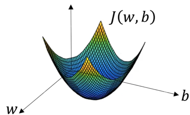
Because the cost function is a convex function, its shape is like the figure below. This is also why we defined the loss function in that form.
What we need to do is initialize values for , then move them in the direction of gradient descent until we find the point with the lowest gradient.
Using as an example, we repeatedly perform the following process: to update , where is the learning-rate parameter. We can see that the larger the slope is, the larger the change in w at each iteration.
In practice, we use the following equations to solve for with gradient descent:
2.4 Computation Graphs
A computation graph performs calculations from left to right to calculate the cost function .
For a flowchart, it is easy to see the derivatives of . Backpropagation works backward from the final output to derive the derivatives of with respect to each intermediate variable and input.
In programs, the usual programming convention is to use dvar to represent the derivative of the final output variable with respect to the variable var.
The approximate code process is as follows:
# 初始化
J = 0
dw1 = 0
dw2 = 0
db = 0
# 遍历数据集
for i = 1 to m
	# 计算损失函数与成本函数
	zi = w1 * x1 + w2 * x2 +b
	ai = 1/(1+exp(-zi))
	J += -[yi * log(ai) + (1 - yi) * log(1-ai)]
	# 求导
	dzi = ai -yi
	dw1 += x1 * dzi
	dw2 += x2 * dzi
	db += dzi
# 解出各参数优化后的值
J/=m
dw1/=m
dw2/=m
db/=m
# 梯度下降
w1=w1-a*dw1
w2=w2-a*dw2
b=b-a*db
2.5 Vectorization
(1) What is vectorization?
Because both the input data and coefficients are column vectors, multiplying these two vectors with a non-vectorized method—that is, implementing it with a for loop—is very slow. A vectorized method, such as using z=np.dot(w,x) in numpy to calculate the dot product of the two vectors, is much faster.
import time

# 向量化
a = np.random.rand(1000000)
b = np.random.rand(1000000)
tic = time.time()
c = np.dot(a,b)
toc = time.time()
print("Vectorized:" + str(1000*(toc-tic))+"ms")
# 非向量化
a = np.random.rand(1000000)
b = np.random.rand(1000000)
tic = time.time()
for i in range(1000000):
	c += a[i]*b[i]
toc = time.time()
print("For Loop:" + str(1000*(toc-tic))+"ms")

# 结果向量化的方法用时1.5ms,for循环方法500ms
The difference is not yet obvious for this small algorithm. However, if training a neural network takes 300 hours with a non-vectorized method but only 1 hour with a vectorized method, the difference becomes very clear.
(2) Vectorizing forward propagation
The purpose of forward propagation is to calculate and .
Vectorization can be implemented as follows: Here, is the input matrix. Each column contains all features of one sample, and there are m columns, meaning m samples in total. is the row vector composed of parameters .
The process above can be represented in a python program as follows:
Z=np.dot(w.T, X) + b(3) Vectorizing gradient calculation
Gradient calculation means calculating , , and .
It can be vectorized as follows:
Vectorize , , and :
Then ,
Expressed in python:
Z=np.dot(w.T,x)+b
A=sigmod(Z)
dZ=A-Y
db=np.sum(dZ)/m
dw=np.dot(X,dZ^T)/m
w=w-a1*dw
b=b-a2*db
(4) Summary To speed up code execution, we used vectorization, meaning that we use numpy to calculate datasets whenever possible instead of using for loops.
Input matrix : samples, each with features
, where
Parameter matrix : one parameter for each feature
Parameter : one parameter for each feature
Linear value , equivalent to a simplified : one calculated value is obtained for each sample
Predicted value : one predicted value for each sample
Loss function : the distance between each sample’s predicted value and labeled value
Cost function : the average of all loss functions
Derivative
Derivative
Derivative
2.6 About numpy and Common Functions
It is best not to use rank 1 arrays such as a=np.random.randn(5). Instead, use an or matrix. In other words, define a row or column vector directly with a=np.random.randn(5,1), or use reshape to change its shape.
If you are unsure of a vector’s dimensions, you can use an assert statement to check them.
assert(a.shape==(5,1))(1) sigmod function
def sigmoid(x):
    """
    参数:
    x -- 任意形状的numpy数组

    返回值:
    s -- sigmoid(x)
    """

    s=1/(1+np.exp(-x))

    return s
(2) Gradient calculation
def sigmoid_derivative(x):
    """
    参数:
    x -- numpy数组

    返回值:
    ds -- 计算的梯度值
    """

    s = 1/(1+np.exp(-x))
    ds = s*(1-s)

    return ds
(3) Reshaping an input image into [width x height x 3, 1]
def image2vector(image):
    """
    参数:
    image -- 特定形状的numpy数组 shape(length, height, depth)

    返回值:
    v -- 向量形式的数组 shape(length*height*depth, 1)
    """

    v = image.reshape(image.shape[0]*image.shape[1]*image.shape[2],1)

    return v
(4) Normalization
def normalizeRows(x):
    """
    参数:
    x -- 一个二维numpy数组 shape(n, m)

    返回值:
    x -- 按行归一化后的numpy矩阵
    """

    # 计算x数组的模
    x_norm = np.linalg.norm(x,ord=2,axis=1,keepdims=True)
    # 用x除以它的模
    x=x/x_norm

return x| Parameter | Description | Calculation |
|---|---|---|
| ord=default | Euclidean norm: | |
| ord=2 | Euclidean norm: | Same as above |
| ord=1 | Taxicab norm: | |
| ord=np.inf | Infinity norm: | $MAX\lvert x_i\rvert$ |
| axis=1 | Process by row vector | |
| axis=0 | Process by column vector | |
| axis=None | Matrix norm |
(5) softmax function
The softmax function is a normalization function used when an algorithm needs to classify two or more classes.
x_{11} & x_{12} & x_{13} & \dots & x_{1n} \\ x_{21} & x_{22} & x_{23} & \dots & x_{2n} \\ \vdots & \vdots & \vdots & \ddots & \vdots \\ x_{m1} & x_{m2} & x_{m3} & \dots & x_{mn} \end{bmatrix} = \begin{bmatrix} \frac{e^{x_{11}}}{\sum_{j}e^{x_{1j}}} & \frac{e^{x_{12}}}{\sum_{j}e^{x_{1j}}} & \frac{e^{x_{13}}}{\sum_{j}e^{x_{1j}}} & \dots & \frac{e^{x_{1n}}}{\sum_{j}e^{x_{1j}}} \\ \frac{e^{x_{21}}}{\sum_{j}e^{x_{2j}}} & \frac{e^{x_{22}}}{\sum_{j}e^{x_{2j}}} & \frac{e^{x_{23}}}{\sum_{j}e^{x_{2j}}} & \dots & \frac{e^{x_{2n}}}{\sum_{j}e^{x_{2j}}} \\ \vdots & \vdots & \vdots & \ddots & \vdots \\ \frac{e^{x_{m1}}}{\sum_{j}e^{x_{mj}}} & \frac{e^{x_{m2}}}{\sum_{j}e^{x_{mj}}} & \frac{e^{x_{m3}}}{\sum_{j}e^{x_{mj}}} & \dots & \frac{e^{x_{mn}}}{\sum_{j}e^{x_{mj}}} \end{bmatrix} = \begin{pmatrix} softmax\text{(first row of x)} \\ softmax\text{(second row of x)} \\ ... \\ softmax\text{(last row of x)} \\ \end{pmatrix} $$ ```python def softmax(x): """ 参数: x -- 一个二维numpy数组 shape(n, m) 返回值: x -- softmax后的numpy矩阵 """ # 计算exp(x) x_exp = np.exp(x) # 创建向量x_sum对x_exp的每一行求和 x_sum = np.sum(x_exp, axis = 1, keepdims = True) # 两者相除计算softmax s = x_exp / x_sum return s ``` **(6) Loss functions** The L1 Loss function is used to evaluate model performance. The larger the loss, the greater the deviation between the predicted and actual values. $$\begin{align*} & L_1(\hat{y}, y) = \sum_{i=0}^m|y^{(i)} - \hat{y}^{(i)}| \end{align*}\tag{6}$$ ```python def L1(yhat, y): """ 参数: yhat -- 长度m的向量(预测值) y -- 长度m的向量(真实值) 返回值: loss -- 上面定义的L1 Loss值 """ loss = np.sum(np.abs(y-yhat)) return loss ``` L2 Loss function. $$\begin{align*} & L_2(\hat{y},y) = \sum_{i=0}^m(y^{(i)} - \hat{y}^{(i)})^2 \end{align*}\tag{7}$$ ```python def L2(yhat, y): """ 参数: yhat -- 长度m的向量(预测值) y -- 长度m的向量(真实值) 返回值: loss -- 上面定义的L2 Loss值 """ loss = np.sum(np.dot(y-yhat,y-yhat)) return loss ``` ## 2.7 Summary **(1) Mathematical process** The purpose of a binary neural network is to take an input $x$ (which may be an image, for example), output a predicted value $\hat y$, and make the predicted value $\hat y$ as close as possible to the actual value $y$: $\hat{y}=P(y=1|x)$ The functional relationship between the predicted output $\hat y$ and input $x$ can be expressed as follows (a sigmod function is added to the linear expression to ensure that the output lies in the [0,1] interval): $$\hat y=\sigma{(wx+b)}$$ Here, $z=wx+b$ and $\sigma(z)=\frac{1}{1+e^{-z}}$ are defined. What we need to do is find the most suitable $w$ and $b$ so that the output $\hat y$ is as close as possible to $y$. Therefore, to measure how close $\hat y$ is to $y$, we define a loss function Loss. As long as the loss function is sufficiently small, $\hat y$ will be sufficiently close to $y$. $$L(\hat y,y)=-y\log{\hat y}-(1-y)\log{(1-\hat y)}$$ When $y=1$, $L(\hat y,y)=-\log{\hat y}$. For $L(\hat y,y)$ to be sufficiently small, $\hat y$ must be sufficiently large, meaning $\hat y\rightarrow y=1$ (because this is a binary problem, $y\in [0,1]$). When $y=0$, $L(\hat y,y)=-\log{(1-\hat y)}$. For $L(\hat y,y)$ to be sufficiently small, $\hat y$ must be sufficiently small, meaning $\hat y\rightarrow y=0$. The above explains why this loss function can describe how close $\hat y$ is to $y$. The loss function above applies to only one sample $x$. A problem generally takes a large number of samples as input; suppose there are $m$. A loss function must be calculated for every sample as described above, and the average of all loss functions is the overall cost function for our input. $$J(w,b)=\frac{1}{m}\sum^{n_x}_{i=1}L(\hat y^{(i)},y^{(i)})$$ The goal of training therefore becomes finding the minimum of $J(w,b)$ and the corresponding $w$ and $b$. Consequently, during each training iteration, we need to differentiate the cost function to obtain $\frac{\partial J}{\partial w}$ and $\frac{\partial J}{\partial b}$, then update $w=w-\alpha \frac{\partial J}{\partial w}$ and $b=b-\frac{\partial J}{\partial w}$ according to the derivatives until we find $J_{min}$ and the corresponding $w$ and $b$. Training is then complete. **(2) Code process** ```python import numpy as np import matplotlib.pyplot as plt import h5py # 常用数据集交互工具,数据集被保存为H5文件 import scipy # 用于图片测试 from PIL import Image from scipy import ndimage # 数据集加载函数 def load_dataset(): train_dataset = h5py.File('datasets/train_catvnoncat.h5', "r") train_set_x_orig = np.array(train_dataset["train_set_x"][:]) # your train set features train_set_y_orig = np.array(train_dataset["train_set_y"][:]) # your train set labels test_dataset = h5py.File('datasets/test_catvnoncat.h5', "r") test_set_x_orig = np.array(test_dataset["test_set_x"][:]) # your test set features test_set_y_orig = np.array(test_dataset["test_set_y"][:]) # your test set labels classes = np.array(test_dataset["list_classes"][:]) # the list of classes train_set_y_orig = train_set_y_orig.reshape((1, train_set_y_orig.shape[0])) test_set_y_orig = test_set_y_orig.reshape((1, test_set_y_orig.shape[0])) return train_set_x_orig, train_set_y_orig, test_set_x_orig, test_set_y_orig, classes # sigmoid函数 def sigmoid(x): """ 参数: x -- numpy数组 返回值: s -- 计算的sigmoid值,sigmoid(z)=1/(1+e^(-z)) """ s = 1/(1+np.exp(-x)) return s # 初始化参数,为w, b创建0向量 def initialize_with_zeros(dim): """ 参数: dim -- w向量的长度 返回值: w -- 初始化的向量, w.shape() -> (dim, 1) b -- 初始化的标量, 偏置值b """ w = np.zeros([dim,1]) b = 0 assert(w.shape == (dim, 1)) assert(isinstance(b, float) or isinstance(b, int)) return w, b # 前向和后向传播函数,计算成本函数和梯度值 def propagate(w, b, X, Y): """ 参数: w -- weights权重, numpy数组 w.shape -> (num_px * num_px * 3, 1) b -- bias偏置, 标量 X -- 数据 X.shape -> (num_px * num_px * 3, number of examples) Y -- 标签向量 (0非猫; 1猫) Y.shape -> (1, number of examples) 返回值: cost -- 成本函数(逻辑回归的负对数) dw -- 损失函数对w的梯度,与w维度相同 db -- 损失函数对b的梯度,与b维度相同 """ m = X.shape[1] # 前向传播(从数据X获得成本函数cost) A = sigmoid(np.dot(w.T,X) + b) cost = - 1/m * np.sum(Y*np.log(A) + (1-Y)*np.log(1-A)) # 后向传播(计算梯度) dw = 1/m * np.dot(X, (A-Y).T) db = 1/m * np.sum(A-Y) assert(dw.shape == w.shape) assert(db.dtype == float) cost = np.squeeze(cost) assert(cost.shape == ()) grads = {"dw": dw, "db": db} return grads, cost # 优化函数,通过梯度下降算法优化w和b def optimize(w, b, X, Y, num_iterations, learning_rate, print_cost = False): """ 参数: w -- weights权重, numpy数组 w.shape -> (num_px * num_px * 3, 1) b -- bias偏置, 标量 X -- 数据 X.shape -> (num_px * num_px * 3, number of examples) Y -- 标签向量 (0非猫; 1猫) Y.shape -> (1, number of examples) num_iterations -- 优化循环的迭代次数 learning_rate -- 学习率 print_cost -- True则每100次打印1次成本函数 返回值: params -- 包括 权重w和偏置b 的字典 grads -- 包括 成本函数对w和b梯度 的字典 costs -- 优化过程中所有的成本函数列表 """ costs = [] for i in range(num_iterations): # 成本函数和梯度计算 grads, cost = propagate(w, b, X, Y) # 从grads字典中获取梯度dw和db dw = grads["dw"] db = grads["db"] # 更新w和b w = w - learning_rate * dw b = b - learning_rate * db # 记录成本函数 if i % 100 == 0: costs.append(cost) # 每100个训练样本打印1次成本函数 if print_cost and i % 100 == 0: print ("Cost after iteration %i: %f" %(i, cost)) params = {"w": w, "b": b} grads = {"dw": dw, "db": db} return params, grads, costs # 预测函数,利用学习到的逻辑回归w和b预测标签 def predict(w, b, X): ''' 参数: w -- weights权重, numpy数组 w.shape -> (num_px * num_px * 3, 1) b -- bias偏置, 标量 X -- 数据 X.shape -> (num_px * num_px * 3, number of examples) 返回值: Y_prediction -- numpy向量包含对所有X样本的预测值 (0/1) ''' m = X.shape[1] Y_prediction = np.zeros((1,m)) w = w.reshape(X.shape[0], 1) # 计算预测值A,预测图片中的是否是猫 A = sigmoid(np.dot(w.T, X) + b) for i in range(A.shape[1]): # 转换概率 A[0,i] 到真实的概率 p[0,i] if A[0,i] < 0.5: Y_prediction[0,i] = 0 else: Y_prediction[0,i] = 1 assert(Y_prediction.shape == (1, m)) return Y_prediction # 综合以上函数,构建逻辑回归模型 def model(X_train, Y_train, X_test, Y_test, num_iterations = 2000, learning_rate = 0.5, print_cost = False): """ 参数: X_train -- 训练数据 (num_px * num_px * 3, m_train) Y_train -- 训练数据标签 (1, m_train) X_test -- 测试数据 (num_px * num_px * 3, m_test) Y_test -- 测试数据标签 (1, m_test) num_iterations -- 迭代次数 learning_rate -- 学习率 print_cost -- 是否打印成本函数 返回值: d -- 包含模型信息的字典 """ # 初始化参数 w, b = initialize_with_zeros(X_train.shape[0]) # 梯度下降 params, grads, costs = optimize(w, b, X_train, Y_train, num_iterations, learning_rate, print_cost) # 从params中获得w和b w, b = params["w"], params["b"] # 预测训练和测试样本 Y_prediction_train = predict(w, b, X_train); Y_prediction_test = predict(w, b, X_test) # 打印训练和测试的准确率 print("train accuracy: {} %".format(100 - np.mean(np.abs(Y_prediction_train - Y_train)) * 100)) print("test accuracy: {} %".format(100 - np.mean(np.abs(Y_prediction_test - Y_test)) * 100)) d = {"costs": costs, "Y_prediction_test": Y_prediction_test, "Y_prediction_train" : Y_prediction_train, "w" : w, "b" : b, "learning_rate" : learning_rate, "num_iterations": num_iterations} return d # 加载数据集 # train_set_x_orig是训练图片数据,train_set_y是训练标签数据 # 每个图像都是正方形(num_px, num_px, 3) train_set_x_orig, train_set_y, test_set_x_orig, test_set_y, classes = load_dataset() # 获取数据集基本参数 m_train = train_set_x_orig.shape[0] # 训练数据数量 m_test = test_set_x_orig.shape[0] # 测试数据数量 num_px = train_set_x_orig.shape[1] # 图片长宽 # 展开训练数据集为一维 train_set_x_flatten = train_set_x_orig.reshape(train_set_x_orig.shape[0],-1).T test_set_x_flatten = test_set_x_orig.reshape(test_set_x_orig.shape[0],-1).T # 数据集标准化处理(将所有像素值[0, 255]映射到[0, 1]) train_set_x = train_set_x_flatten/255 test_set_x = test_set_x_flatten/255 # 运行model进行训练 d = model(train_set_x, train_set_y, test_set_x, test_set_y, num_iterations = 20000, learning_rate = 0.005, print_cost = True) # 查看某张图片的预测结果 index = 1 plt.imshow(test_set_x[:,index].reshape((num_px, num_px, 3))) print ("y = " + str(test_set_y[0,index]) + ", you predicted that it is a \"" + classes[int(d["Y_prediction_test"][0,index])].decode("utf-8") + "\" picture.") # 画出学习曲线 costs = np.squeeze(d['costs']) plt.plot(costs) plt.ylabel('cost') plt.xlabel('iterations (per hundreds)') plt.title("Learning rate =" + str(d["learning_rate"])) plt.show() ``` # III. Neural Networks ## 3.1 Representing a Neural Network A typical neural network includes an input layer, hidden layer, output layer, and output value. > Hidden layer: In the training set, we do not know the values of these nodes. We can see the input and output values, but we cannot see the intermediate values during training, so it is called the hidden layer.  The figure above shows a standard two-layer neural network (the input layer is not counted as a standard layer), also known as a single-hidden-layer neural network. In the network above, the input layer can also be denoted by $a^{[0]}$, where $a^{[0]}=X$. The intermediate layer can be denoted by $a^{[1]}$, where $a^{[1]}=[a^{[1]}_1 a^{[1]}_2 \cdots a^{[1]}_n]$. The output layer can be denoted by $a^{[2]}$. We use square brackets to indicate the layer number in the neural network. The hidden and output layers have their own parameters, denoted by $w^{[1]}, b^{[1]}$ and $w{[2]}, b{[2]}$, respectively. ## 3.2 Neural Network Computation The computation process of a neural network is the regression calculation from the previous section stacked multiple times. The figure below shows the logistic regression process discussed in the previous section. 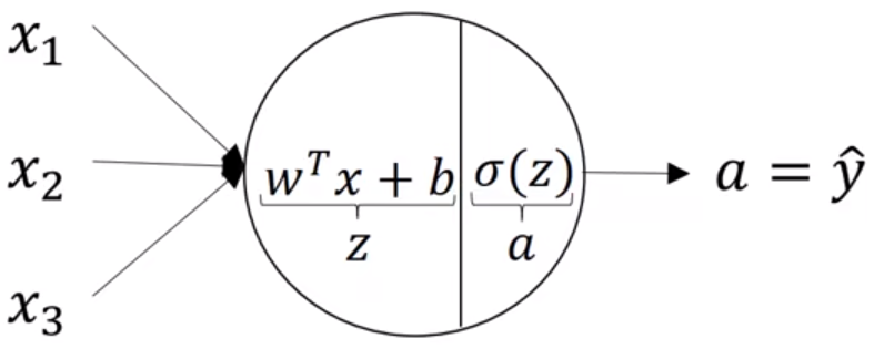 In a two-layer neural network, it corresponds to the part shown below (between the hidden and input layers). Every hidden-layer unit uses the same computation process. 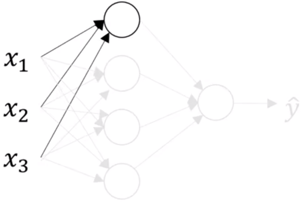 The computation between the output and hidden layers is also similar to that between the hidden and input layers. The only difference is that the $a^{[1]}$ calculated by the hidden layer is treated as the input for the regression calculation. The computation process of a two-layer neural network can be expressed mathematically as follows: $$z^{[1]}=W^{[1]}x+b^{[1]}$$ $$a^{[1]}=\sigma (z^{[1]})$$ $$z^{[2]}=W^{[2]}a^{[1]}+b^{[2]}$$ $$a^{[2]}=\sigma (z^{[2]})$$ ## 3.3 Activation Functions **(1) The $\sigma$ function** The activation functions mentioned earlier all use the $\sigma$ function [0, 1], but this function is almost never used in practice. 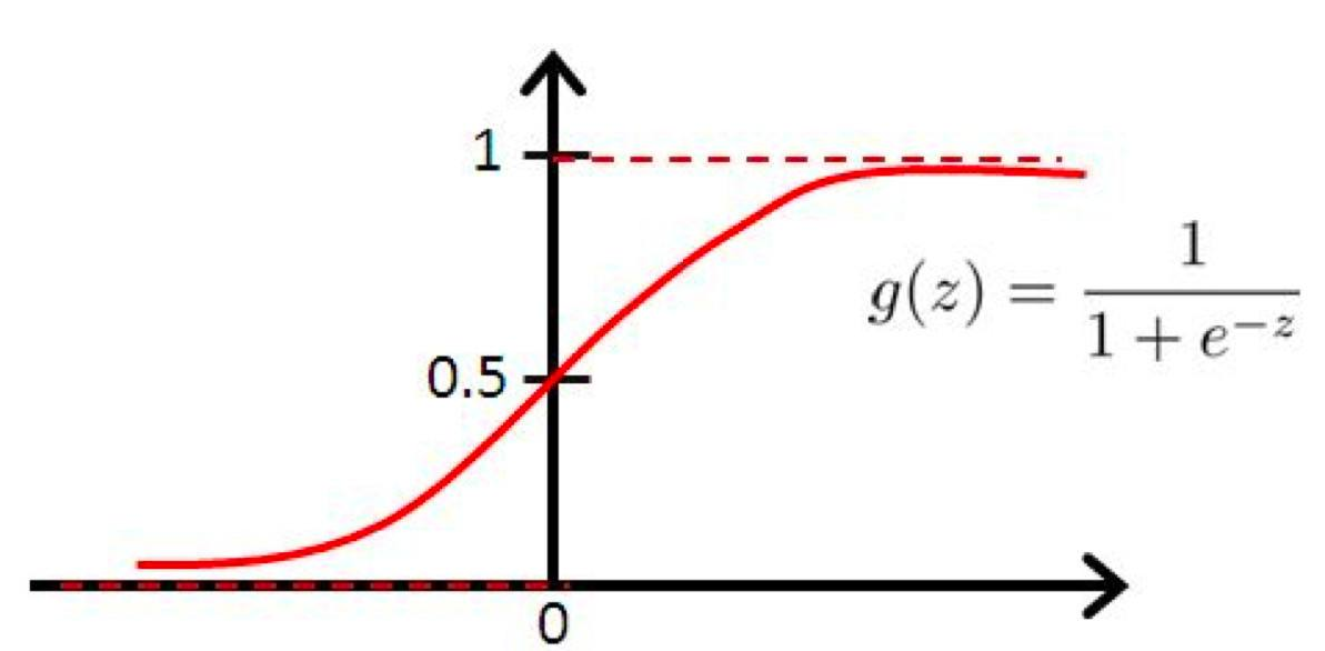 **(2) The tanh function** More generally, we use other nonlinear functions, such as the $tanh = \frac{e^z-e^{-z}}{e^z+e^{-z}}$ function [-1, 1]. It has been shown that using tanh as the hidden-layer activation function almost always works better than $\sigma$. For the output layer, because $\hat y \in [0, 1]$, the $\sigma$ function works better. 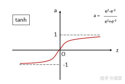 **(3) ReLU function** However, for both $\sigma$ and tanh, we can see that when z is very large or very small, the slope of the activation function is very small. This severely affects how quickly gradient descent finds the optimal solution. The rectified linear unit ReLU was therefore proposed. 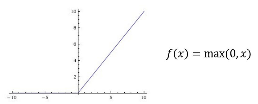 There is also a leaky rectified linear unit, Leaky ReLU, where a is nonzero when z<0. 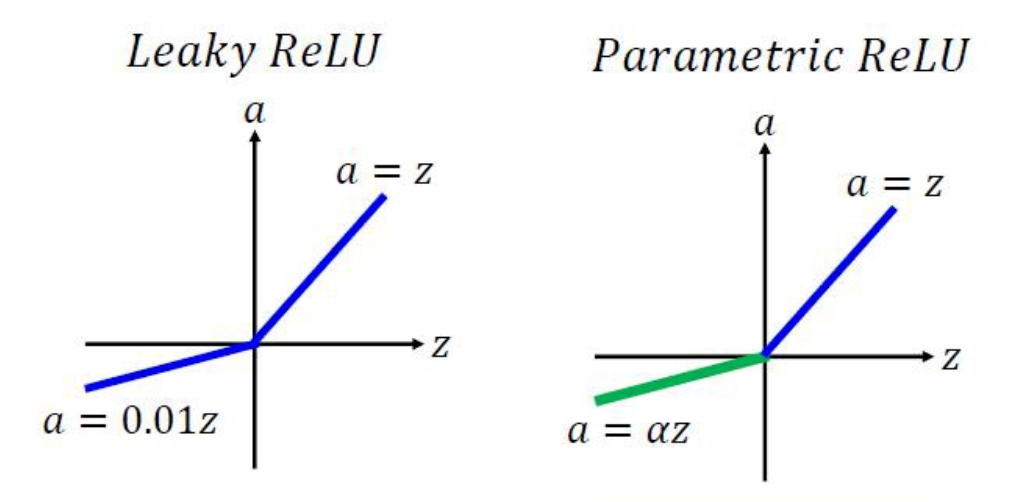 **(4) Why nonlinear activation functions are needed** If machine learning is not used, the forward computation process of the two-layer neural network described earlier is: $$z^{[1]}=W^{[1]}x+b^{[1]}$$ $$a^{[1]}=\sigma (z^{[1]})$$ $$z^{[2]}=W^{[2]}a^{[1]}+b^{[2]}$$ $$a^{[2]}=\sigma (z^{[2]})$$ Let $a^{[1]}=z^{[1]}$. The computation process can then be written as follows: $$z^{[2]}=W^{[2]}z^{[1]}+b^{[2]}=W^{[2]}(W^{[1]}x+b^{[1]})+b^{[2]}=W'x+b'$$ After simplification, $z^{[2]}$ and x can be represented linearly. In other words, no matter how many layers the network has, its output and input can be represented by a single linear function, so the role of the neural network cannot be realized. Activation functions are therefore essential. From another perspective, a neural network simulates the signal transmission process of neurons. Activation functions such as ReLU simulate a neuron's firing threshold: a signal is sent to the next neuron only when electrical stimulation reaches a certain threshold. Likewise, an activation function produces output only when the threshold is reached; otherwise, its output is 0. This also removes certain unimportant sample features and prevents phenomena such as overfitting. **(5) Derivatives of activation functions** For the sigmod function, $g(z)=\frac{1}{1+e^{-z}}$, it is easy to calculate that $\frac{d}{dz}g(z)=\frac{1}{1+e^{-z}}] (1-\frac{1}{1+e^{-z}})=g(z)(1-g(z))$. - When z->+∞, g(z)->1 and g'(z)->0; - When z->-∞, g(z)->0 and g'(z)->0 - When z=0, g(z)=0.5 and g'(z)=0.25 For the tanh function, $g(z)=\frac{e^z-e^{-z}}{e^z+e^{-z}}$, it is easy to calculate that $\frac{d}{dz}g(z)=1-(tanh(z))^2$. - When z->+∞, g(z)->1 and g'(z)->0; - When z->-∞, g(z)->-1 and g'(z)->0 - When z=0, g(z)=0 and g'(z)=1 For the ReLU function, $g(z)=max(0,z)$, it is easy to calculate: $g'(z)=0, if z<0$ $g'(z)=1, if z>=0$ (When z=0, the derivative can be set to 1 in the program to avoid the non-differentiability problem.) ## 3.4 Gradient Descent for Neural Networks For a neural network, we have the following parameters: $w^{[1]}, b^{[1]}, w^{[2]}, b^{[2]}$ The loss function we calculate is: $J(w^{[1]}, b^{[1]}, w^{[2]}, b^{[2]})=\frac{1}{m} \sum^n_{i=1}l(\hat y, y)$ The gradient descent process repeats the following steps: 1. Calculate the predicted value $\hat y$ 2. Calculate the derivatives: $d(w^{[1]})=\frac{\partial J}{\partial w^{[1]}}$, $d(b^{[1]})=\frac{\partial J}{\partial b^{[1]}}$ 3. Update the parameters: $w^{[1]}=w^{[1]}-\alpha \frac{\partial J}{\partial w^{[1]}}$, $b^{[1]}=b^{[1]}-\alpha \frac{\partial J}{\partial b^{[1]}}$ After vectorization, backpropagation is calculated as follows: $$dZ^{[2]}=A^{[2]}-Y$$ $$dW^{[2]}=\frac{1}{m}dZ^{[2]}A^{[1]T}$$ $$db^{[2]}=dZ^{[2]}$$ $$dZ^{[1]}=W^{[2]T}dZ^{[2]}*g^{[1]'}(Z^{[1]})$$ $$dW^{[1]}=\frac{1}{m}dZ^{[1]}X^T$$ $$db^{[1]}=dZ^{[1]}$$ ## 3.5 Parameter Initialization The weight parameters of every layer in a neural network must be initialized. However, simply initializing them to 0 makes the neural network completely ineffective, so we need random initialization. We can set: W[1]=np.random.randn((2,2))\*0.01 b[1]=np.zero((2,1)) W[1]=np.random.randn((1,2))\*0.01 b[1]=0 We multiply by 0.01 because we prefer the weights to be as small as possible. This also makes z smaller and more likely to fall in a region where the activation function has a large slope, allowing the neural network to regress more quickly. ## 3.6 Code Implementation **(1) Installing packages** Some necessary packages need to be imported when implementing the neural network: - numpy: a basic scientific computing package - sklearn: provides simple and effective tools for data mining and data analysis - matplotlib: a plotting tool **(2) Neural network** Steps for building a neural network: 1. Define the neural network structure (number of input units, number of hidden units, and so on) 2. Initialize the model parameters 3. Loop: - Implement forward propagation - Calculate the loss function - Use backpropagation to obtain the gradients - Use gradient descent to update the parameters 1. Define the neural network structure ```python # GRADED FUNCTION: layer_sizes def layer_sizes(X, Y): """ 参数: X -- 输入数据集,shape(input size, number of examples) Y -- 标签,shape(output size, number of examples) 返回值: n_x -- 输入层的大小 n_h -- 隐藏层的大小 n_y -- 输出层的大小 """ n_x = X.shape[0] n_h = 4 n_y = Y.shape[0] return (n_x, n_h, n_y) ``` 2. Initialize the model parameters ```python def initialize_parameters(n_x, n_h, n_y): """ 参数: n_x -- 输入层的大小 n_h -- 隐藏层的大小 n_y -- 输出层的大小 返回值: params -- python字典包含以下参数: W1 -- 权重矩阵,shape (n_h, n_x) b1 -- 偏置向量,shape (n_h, 1) W2 -- 权重矩阵,shape (n_y, n_h) b2 -- 偏置向量,shape (n_y, 1) """ np.random.seed(2) W1 = np.random.randn(n_h, n_x) b1 = np.zeros((n_h, 1)) W2 = np.random.randn(n_y, n_h) b2 = np.zeros((n_y, 1)) assert (W1.shape == (n_h, n_x)) assert (b1.shape == (n_h, 1)) assert (W2.shape == (n_y, n_h)) assert (b2.shape == (n_y, 1)) parameters = {"W1": W1, "b1": b1, "W2": W2, "b2": b2} return parameters ``` 3. Forward propagation ```python def forward_propagation(X, parameters): """ 参数: X -- 输入数据,size (n_x, m) parameters -- 包含所有参数的字典 (上面初始化函数的输出) 返回值: A2 -- 第二次激活后的输出 cache -- 包含 "Z1", "A1", "Z2", "A2" 的字典 """ # 从字典 "parameters" 中获取各参数 W1 = parameters["W1"] b1 = parameters["b1"] W2 = parameters["W2"] b2 = parameters["b2"] # 前向传播计算A2 Z1 = np.dot(W1, X) + b1 A1 = np.tanh(Z1) Z2 = np.dot(W2, A1) + b2 A2 = np.tanh(Z2) assert(A2.shape == (1, X.shape[1])) cache = {"Z1": Z1, "A1": A1, "Z2": Z2, "A2": A2} return A2, cache ``` 4. Calculate the loss function ```python def compute_cost(A2, Y, parameters): """ 参数: A2 -- 第二次激活函数的输出,shape (1, number of examples) Y -- 真值向量,shape (1, number of examples) parameters -- 包含所有参数的字典 返回值: cost -- 损失函数 """ m = Y.shape[1] # 样本的数量 # 计算损失函数 logprobs = np.multiply(np.log(A2), Y) + np.multiply((1 - Y), np.log(1 - A2)) cost = - np.sum(logprobs) / m cost = np.squeeze(cost) # 保证损失函数的维度是我们想要的,例如把[[6]]变成6 assert(isinstance(cost, float)) return cost ``` 5. Backpropagation ```python def backward_propagation(parameters, cache, X, Y): """ 参数: parameters -- 包含所有参数的字典 cache -- 包含 "Z1", "A1", "Z2", "A2" 的字典 X -- 输入数据,shape (2, number of examples) Y -- 真值向量,shape (1, number of examples) 返回值: grads -- 包含所有参数的梯度值的字典 """ m = X.shape[1] # 从字典 "parameters" 中获取 W1, W2 W1 = parameters["W1"] W2 = parameters["W2"] # 从字典 "cache" 中获取 A1, A2 A1 = cache["A1"] A2 = cache["A2"] # 反向传播: 计算 dW1, db1, dW2, db2. dZ2 = A2 - Y dW2 = 1/m * np.dot(dZ2, A2.T) db2 = 1/m * np.sum(dZ2, axis = 1, keepdims = True) dZ1 = np.multiply(np.dot(W2.T, dZ2), (1 - np.power(A1, 2))) dW1 = 1/m * np.dot(dZ1, X.T) db1 = 1/m * np.sum(dZ1, axis = 1, keepdims = True) grads = {"dW1": dW1, "db1": db1, "dW2": dW2, "db2": db2} return grads ``` 6. Update the parameters ```python def update_parameters(parameters, grads, learning_rate = 1.2): """ 参数: parameters -- 包含所有参数的字典 grads -- 包含所有梯度的字典 返回值: parameters -- 包含所有更新后的参数的字典 """ # 从字典 "parameters" 中获取 W1, W2, b1, b2 W1 = parameters["W1"] b1 = parameters["b1"] W2 = parameters["W2"] b2 = parameters["b2"] # 从字典 "grads" 中获取梯度值 dW1, dW2, db1, db2 dW1 = grads["dW1"] db1 = grads["db1"] dW2 = grads["dW2"] db2 = grads["db2"] # 更新每个参数 W1 = W1 - learning_rate * dW1 b1 = b1 - learning_rate * db1 W2 = W2 - learning_rate * dW2 b2 = b2 - learning_rate * db2 parameters = {"W1": W1, "b1": b1, "W2": W2, "b2": b2} return parameters ``` 7. Integrate the functions ```python def nn_model(X, Y, n_h, num_iterations = 10000, print_cost=False): """ 参数: X -- 数据集,shape (2, number of examples) Y -- 标签,shape (1, number of examples) n_h -- 隐藏层的大小 num_iterations -- 梯度下降循环的迭代次数 print_cost -- True则每1000次迭代打印cost 返回值: parameters -- 模型学习到的参数,可以被用来预测 """ np.random.seed(3) n_x = layer_sizes(X, Y)[0] n_y = layer_sizes(X, Y)[2] # 初始化参数, 获取 W1, b1, W2, b2 # Inputs: "n_x, n_h, n_y". Outputs = "W1, b1, W2, b2, parameters". parameters = initialize_parameters(n_x, n_h, n_y) W1 = parameters["W1"] b1 = parameters["b1"] W2 = parameters["W2"] b2 = parameters["b2"] # 梯度下降循环 for i in range(0, num_iterations): # 前向计算 # Inputs: "X, parameters". Outputs: "A2, cache". A2, cache = forward_propagation(X, parameters) # 损失函数 # Inputs: "A2, Y, parameters". Outputs: "cost". cost = compute_cost(A2, Y, parameters) # 反向传播 # Inputs: "parameters, cache, X, Y". Outputs: "grads". grads = backward_propagation(parameters, cache, X, Y) # 梯度下降参数更新 # Inputs: "parameters, grads". Outputs: "parameters". parameters = update_parameters(parameters, grads) # 每1000次迭代打印cost if print_cost and i % 1000 == 0: print ("Cost after iteration %i: %f" %(i, cost)) return parameters ``` 8. Prediction ```python def predict(parameters, X): """ 参数: parameters -- 包含训练好的参数的字典 X -- 输入数据,size (n_x, m) 返回值: predictions -- 模型的预测结果向量 """ # 计算前向传播的概率,并按概率0.5为界限进行二分分类 A2, cache = forward_propagation(X, parameters) predictions = np.round(A2) return predictions ``` # IV. Deep Neural Networks ## 4.1 Forward Propagation **(1) Mathematical calculations** $$z^{[1]}=W^{[1]}x+b^{[1]}$$ $$a^{[1]}=g(z^{[1]})$$ $$z^{[2]}=W^{[2]}a^{[1]}+b^{[2]}$$ $$a^{[2]}=g(z^{[2]})$$ $$\cdots$$ $$z^{[l]}=W^{[l]}a^{[l-1]}+b^{[l]}$$ $$a^{[l]}=g(z^{[l]})$$ **(2) Vectorization** $$Z^{[l]}=W^{[l]}A^{[l-1]}+b^{[l]}$$ $$A^{[l]}=g(Z^{[l]})$$ ## 4.2 Checking Matrix Dimensions **(1) Derivation** For the computation process: $$Z^{[l]}=W^{[l]}A^{[l-1]}+b^{[l]}$$ Because the number of rows in $Z^{[l]}$ equals the number of neuron units $n^{l}$ in each layer and the number of columns equals the number of samples $m$, the dimensions of $Z^{[l]}$ are $(n^{[l]}, m)$. $A^{[l-1]}$ is obtained by applying the activation function to $Z^{[l-1]}$, so it has the same dimensions as $Z^{[l-1]}$: $(n^{[l-1]},1)$. According to the rules of matrix computation, the dimensions of $W^{[l]}$ are $(n^{[l]}, n^{[l-1]})$. The dimensions of $b$ should be the same as those of $Z^{[l]}$, namely $(n^{[l]}, m)$. However, because of python's broadcasting rules, the dimensions of $b$ in a program are usually $(n^{[l]}, 1)$. **(2) Summary of dimensions** $$W^{[l]}:(n^{[l]}, n^{[l-1]})$$ $$b^{[l]}:(n^{[l]}, 1)$$ $$dW^{[l]}:(n^{[l]}, n^{[l-1]})$$ $$db^{[l]}:(n^{[l]}, 1)$$ ## 4.3 Parameters and Hyperparameters The parameters used in deep learning include: - Weights: $W^{[l]}$ - Biases: $b^{[b]}$ The hyperparameters include: - Learning rate: $\alpha$ - Number of iterations - Number of hidden layers: L - Number of hidden-layer units: $n^{[l]}$ - Choice of activation function All hyperparameters can determine the final parameters W and b to some extent. We can set different hyperparameters and observe changes in the cost function to determine whether the current hyperparameters are the most suitable. Hyperparameters generally need to be tested repeatedly to find the best values for the current problem. ## 4.4 Implementing the Key Steps **(1) Parameter initialization** ```python def initialize_parameters_deep(layer_dims): """ 参数: layer_dims -- 包含每一层维度的列表 返回值: parameters -- 包含 "W1", "b1", ..., "WL", "bL" 的字典 Wl -- 权值矩阵,shape (layer_dims[l], layer_dims[l-1]) bl -- 偏置向量,shape (layer_dims[l], 1) """ np.random.seed(3) parameters = {} L = len(layer_dims) # 神经网络的层数 for l in range(1, L): parameters["W" + str(l)] = np.random.randn(layer_dims[l], layer_dims[l - 1]) * 0.01 parameters["b" + str(l)] = np.zeros((layer_dims[l], 1)) assert(parameters['W' + str(l)].shape == (layer_dims[l], layer_dims[l-1])) assert(parameters['b' + str(l)].shape == (layer_dims[l], 1)) return parameters ``` **(2) Forward propagation linear-activation module** ```python def linear_activation_forward(A_prev, W, b, activation): """ 参数: A_prev -- 上一层激活后的结果 (或输入数据),shape(上一层单元数, 样本数) W -- 权值矩阵,shape (当前层单元数, 上一层单元数) b -- 偏置向量,shape (当前层单元数, 1) activation -- 本层使用的激活函数, 字符串格式: "sigmoid" or "relu" 返回值: A -- 激活函数后的输出 cache -- 包含 "linear_cache" and "activation_cache" 的字典,便于反向传播的计算 """ if activation == "sigmoid": # Inputs: "A_prev, W, b". Outputs: "A, activation_cache". ### START CODE HERE ### (≈ 2 lines of code) Z = np.dot(W, A_prev) + b A, activation_cache = sigmoid(Z) ### END CODE HERE ### elif activation == "relu": # Inputs: "A_prev, W, b". Outputs: "A, activation_cache". ### START CODE HERE ### (≈ 2 lines of code) Z = np.dot(W, A_prev) + b A, activation_cache = relu(Z) ### END CODE HERE ### assert (A.shape == (W.shape[0], A_prev.shape[1])) cache = (linear_cache, activation_cache) return A, cache ``` **(3) L-layer neural network** ```python def L_model_forward(X, parameters): """ 参数: X -- 输入数据,shape (input size, number of examples) parameters -- 初始化参数,initialize_parameters_deep()的输出 返回值: AL -- 激活函数的输出 caches -- 包括 每层linear_relu_forward()的cache (一共L-1个, 索引从0到L-2) linear_sigmoid_forward()的cache (只有一个, 索引为L-1) """ caches = [] A = X L = len(parameters) // 2 # 神经网络的层数 # 实现 [LINEAR -> RELU]*(L-1). 添加 "cache" 到 "caches" 列表. for l in range(1, L): A_prev = A A, cache = linear_activation_forward(A_prev, parameters["W" + str(l)], parameters["b" + str(l)], "relu") caches.append(cache) # 实现 LINEAR -> SIGMOID. 添加 "cache" 到 "caches" 列表. AL, cache = linear_activation_forward(A, parameters["W" + str(L)], parameters["b" + str(L)], "sigmoid") caches.append(cache) assert(AL.shape == (1,X.shape[1])) return AL, caches ``` **(4) Cost function** ```python def compute_cost(AL, Y): """ 参数: AL -- 与输入的标签匹配的预测值向量, shape(1, number of examples) Y -- 真值标签向量 (例如: 不是猫为0,猫为1), shape (1, number of examples) 返回值: cost -- 成本函数 """ m = Y.shape[1] # 根据al, y计算成本函数 cost = -1 / m * np.sum(Y * np.log(AL) + (1-Y) * np.log(1-AL),axis=1,keepdims=True) cost = np.squeeze(cost) # 保证成本函数的向量是我们想要的,例如[[17]]变成17 assert(cost.shape == ()) return cost ``` **(5) Backpropagation through the linear part** ```python def linear_backward(dZ, cache): """ 参数: dZ -- 第L层的线性输出的梯度 cache -- (A_prev, W, b)组成的元组,来自当前层的前向传播 返回值: dA_prev -- 上一层激活函数后的梯度 dW -- W的梯度 db -- b的梯度 """ A_prev, W, b = cache m = A_prev.shape[1] dW = 1/m * np.dot(dZ, A_prev.T) db = 1/m * np.sum(dZ,axis=1, keepdims=True) dA_prev = np.dot(W.T, dZ) assert (dA_prev.shape == A_prev.shape) assert (dW.shape == W.shape) assert (db.shape == b.shape) return dA_prev, dW, db ``` **(6) Backpropagation through the linear-activation part** ```python def linear_activation_backward(dA, cache, activation): """ 参数: dA -- 当前层激活后的梯度 cache -- (linear_cache, activation_cache)组成的元组,为了反向传播计算更快 activation -- 当前层所用的激活函数, 以字符串格式存储: "sigmoid" or "relu" 返回值: dA_prev -- 上一层激活后的梯度 dW -- W的梯度 db -- b的梯度 """ linear_cache, activation_cache = cache if activation == "relu": dZ = relu_backward(dA, activation_cache) dA_prev, dW, db = linear_backward(dZ, linear_cache) elif activation == "sigmoid": dZ = sigmoid_backward(dA, activation_cache) dA_prev, dW, db = linear_backward(dZ, linear_cache) return dA_prev, dW, db ``` **(7) Backpropagation through the linear model** ```python def L_model_backward(AL, Y, caches): """ 参数: AL -- 概率向量, 前向传播的输出(L_model_forward()) Y -- 数据集真值向量 caches -- 列表包括 linear_activation_forward() 函数的cache (是caches[l], for l in range(L-1) i.e l = 0...L-2) linear_activation_forward() 函数的cache (是caches[L-1]) 返回值: grads -- 梯度的字典 grads["dA" + str(l)] = ... grads["dW" + str(l)] = ... grads["db" + str(l)] = ... """ grads = {} L = len(caches) # 层数 m = AL.shape[1] Y = Y.reshape(AL.shape) # 此行后,Y与YL相同 # 初始化反向传播 dAL = - (np.divide(Y, AL) - np.divide(1 - Y, 1 - AL)) # 第L层梯度 (SIGMOID -> LINEAR). 输入: "AL, Y, caches". 输出: "grads["dAL"], grads["dWL"], grads["dbL"] current_cache = caches[L-1] grads["dA" + str(L)], grads["dW" + str(L)], grads["db" + str(L)] = linear_activation_backward(dAL, current_cache, activation = "sigmoid") for l in reversed(range(L - 1)): # l层梯度 (RELU -> LINEAR) # 输入: "grads["dA" + str(l + 2)], caches". 输出: "grads["dA" + str(l + 1)] , grads["dW" + str(l + 1)] , grads["db" + str(l + 1)] current_cache = caches[l] dA_prev_temp, dW_temp, db_temp = linear_activation_backward(grads["dA" + str(l+2)], current_cache, activation = "relu") grads["dA" + str(l + 1)] = dA_prev_temp grads["dW" + str(l + 1)] = dW_temp grads["db" + str(l + 1)] = db_temp return grads ``` **(8) Parameter updates** ```python def update_parameters(parameters, grads, learning_rate): """ 参数: parameters -- 包含所有参数的python字典 grads -- 包含所有梯度的字典, L_model_backward 函数的输出 learning_rate -- 学习率 返回值: parameters -- 包含所有更新后参数的字典 parameters["W" + str(l)] = parameters["W" + str(l)] - learning_rate * grads["dW" + str(l + 1)] parameters["b" + str(l)] = parameters["b" + str(l)] - learning_rate * grads["db" + str(l + 1)] """ L = len(parameters) // 2 # 神经网络的层数 # 参数更新 for l in range(L): parameters["W" + str(l + 1)] -= learning_rate * grads["dW" + str(l + 1)] parameters["b" + str(l + 1)] -= learning_rate * grads["db" + str(l + 1)] return parameters ```
Comments