LabVIEW Study Notes (X): Case Structures

LabVIEW Study Notes: LabVIEW Study Notes (I): Basic Introduction LabVIEW Study Notes (II): Filter Experiment LabVIEW Study Notes (III): Basic Controls LabVIEW Study Notes (IV): Dynamic Data Types LabVIEW Study Notes (V): Comprehensive Data Type Experiment LabVIEW Study Notes (VI): While Loops and For Loops LabVIEW Study Notes (VII): Variables and Shift Registers LabVIEW Study Notes (VIII): Property Nodes LabVIEW Study Notes (IX): Arrays and Clusters LabVIEW Study Notes (X): Case Structures Other Experiment Records

---

Case Structures

1. Case structures are similar to if…else… and switch structures in C and are mainly used to select among branches of program logic.
2. A case structure contains two or more subdiagrams or cases. Only one case executes at a time.
3. Right-click the case structure border to add, duplicate, delete, reorder, or select the default case.

Input and Output Tunnels

1. Multiple input/output tunnels can be created.
2. Input data is available to all cases.
3. Each case must define its own output tunnels.
4. By default, the case selector is Boolean. When it is true, the contents of the True case execute; when it is false, the contents of the False case execute. The case selector can also receive input from controls such as arrays and enums.

Experiment

Task Requirements

1. Generate a signal with a configurable frequency and waveform type.
2. Use a sufficiently high sampling rate to generate and display a waveform, then generate a waveform with an adjustable sampling rate and compare them.
3. Display the waveform and signal spectrum.

Implementation

1. Signal generation and display are continuous processes, so use a loop.
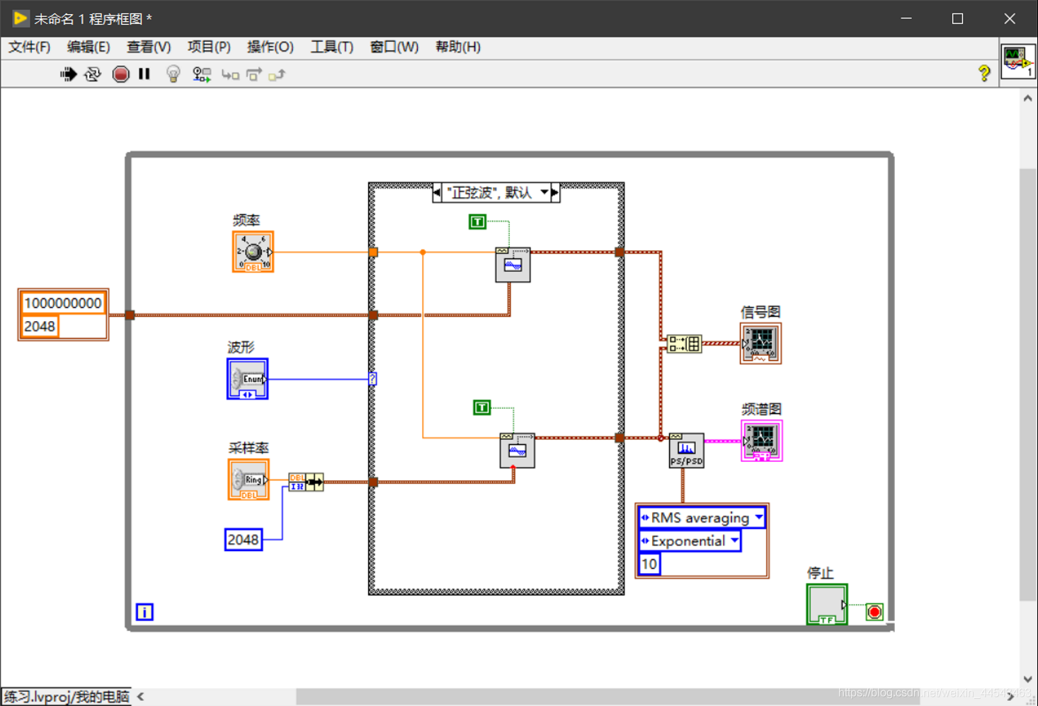
2. Because the signal’s waveform type is configurable, insert an enum variable on the front panel for this setting. Different enum values should generate different waveforms, so use a case structure to select the appropriate waveform.
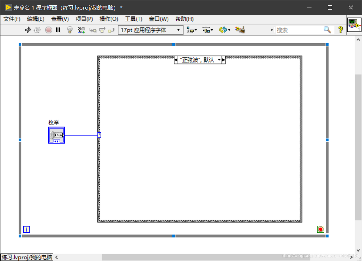
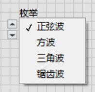
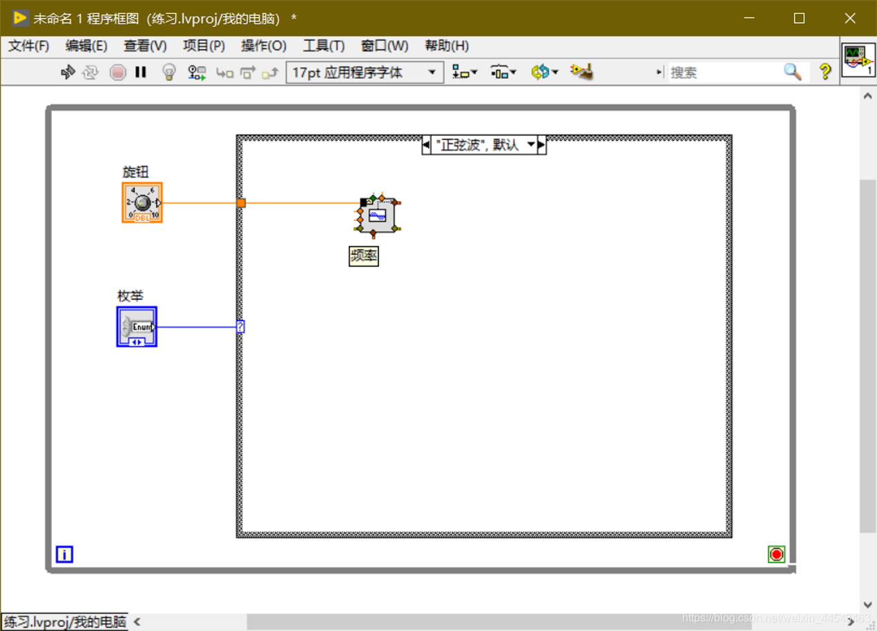
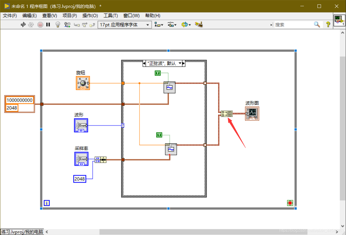
3. First configure the first waveform, the sine wave, by adding a sine waveform generation control to the block diagram. (1) Configure the waveform: insert a knob on the front panel to adjust the frequency, return to the block diagram, and wire it to the frequency input of the sine waveform generation control. 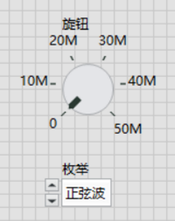(2) Configure the sampling information: add a constant at the corresponding input and increase the sampling rate to generate a sine signal with a sufficiently high sampling rate.
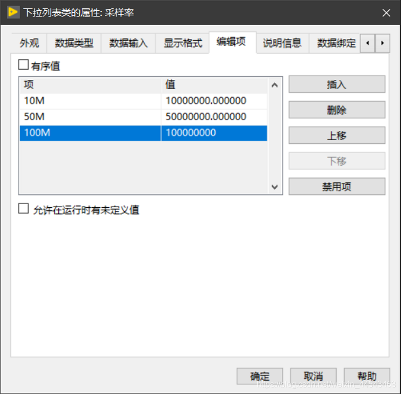
4. Generate the sampled signal: add another sine waveform generation control to generate the sampled signal. On the front panel, add a text drop-down list control to set the sampling rate (the data type is DBL, and the sampling rates are shown in the figure). Use Bundle to bundle the sampling rate and number of samples, then pass the bundle to the sampling information input of the sine waveform generation control. Configure the other inputs in the same way as for the sine waveform above.
5. Display the signals: because two signals must be displayed, use Build Array to combine them into an array and pass it to the waveform graph.
6. Measure the signal: add FFT Power Spectrum and PSD (under Signal Processing - Waveform Measurements). Connect the sampled signal to the time signal input. Create a constant for the averaging parameters input and select RMS averaging. Then add a waveform graph control on the front panel to display the spectrum.
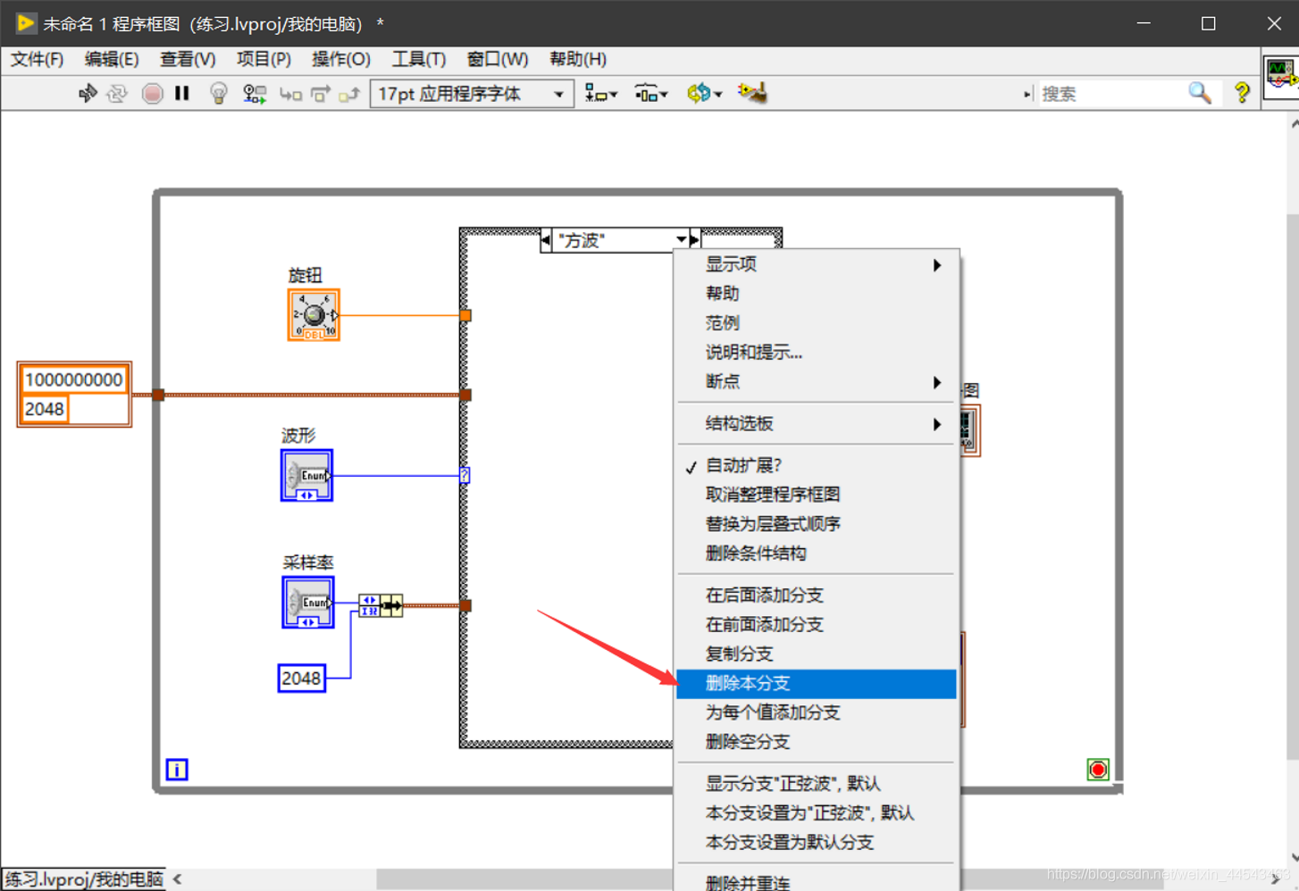
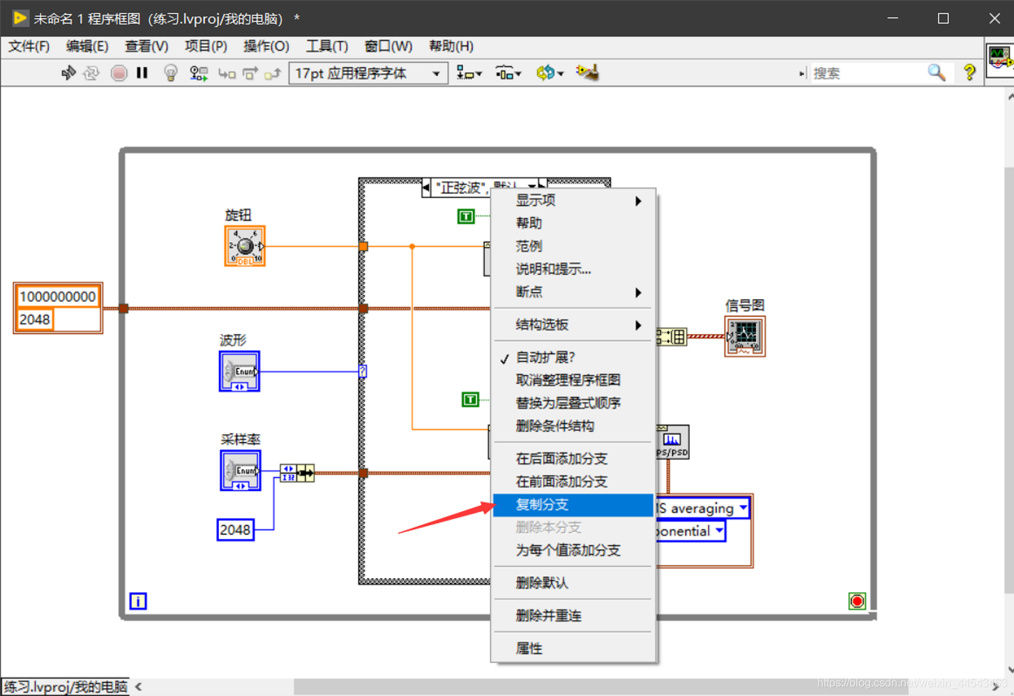
7. Configure other waveforms: first delete the square-wave case from the case structure, then duplicate the sine-wave case and replace the sine waveform generation control inside the case structure with a square-wave generation control. (Other waveforms follow a similar procedure.)
8. Add a Stop button, adjust the waveform graph’s horizontal-axis display range, and finish styling the interface. The program is then complete. 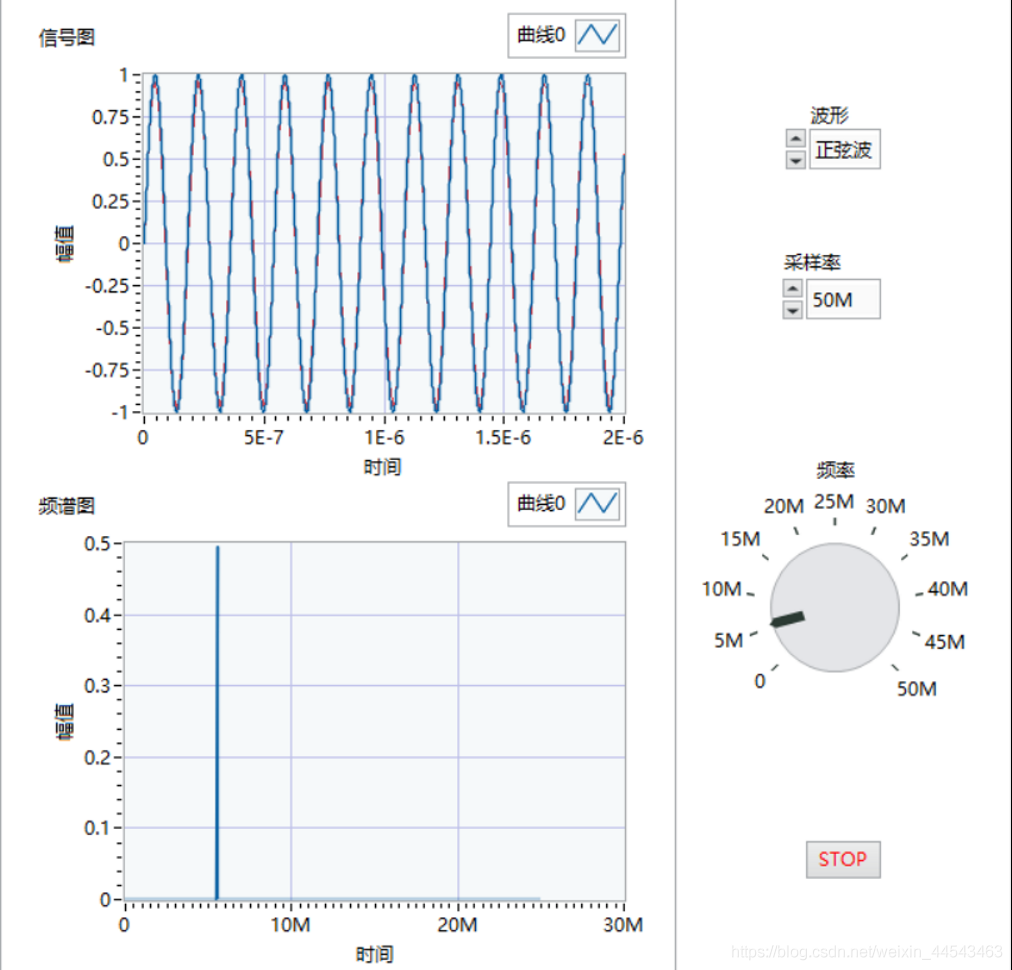When the sampling rate is sufficiently high, the waveform signal and the sampling rate almost completely overlap. 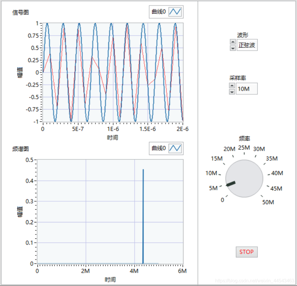When the sampling rate is low, obvious distortion occurs.