[Paper Notes] FFB6D

I. Overview

This method treats the RGB image and depth information as two data sources; the key is how to combine them effectively.

Our key insight is that appearance information in the RGB image and geometry information from the depth image are two complementary data sources, and it still remains unknown how to fully leverage them.

By building bidirectional fusion channels in every layer of the RGB and depth feature extraction networks, the two networks can use each other’s local and global features.

Specifically, at the representation learning stage, we build bidirectional fusion modules in the full flow of the two networks, where fusion is applied to each encoding and decoding layer . In this way, the two networks can leverage local and global complementary information from the other one to obtain better representations.

At the network output stage, a keypoint selection algorithm that considers texture and geometry information is designed, which simplifies keypoint localization and enables precise pose estimation.

Moreover , at the output representation stage, we designed a simple but effective 3D keypoints selection algorithm considering the texture and geometry information of objects, which simplifies keypoint localization for precise pose estimation.

II. FFB6D Pipeline Diagram

Overall pipeline

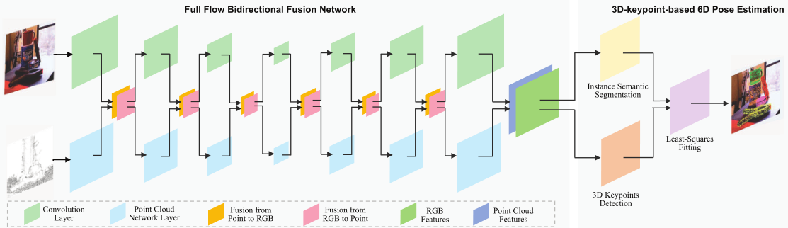
A CNN and a point cloud network represent RGB and the point cloud respectively, with bidirectional fusion modules bridging every corresponding layer of the two networks. The extracted per-point features are fed into an instance segmentation module and a 3D keypoint voting module, and the object’s 6D pose is finally regressed.

Pixel-to-point cloud fusion module

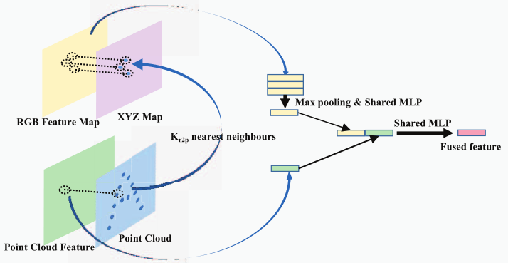
RGB feature map part: for each point in the point cloud, find its spatial nearest neighbors, look up the corresponding RGB feature maps for those points, and produce one RGB feature map from these features through pooling and a shared multilayer perceptron.

Point cloud feature part: extract point cloud features directly.

The two are combined into a new set of RGB–point cloud features and passed to the next layer.

Point cloud-to-pixel fusion module

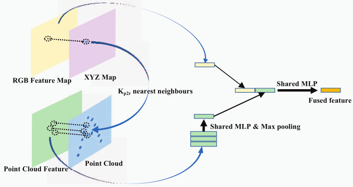
This is the dual of pixel-to-point cloud processing.

III. Implementation Details

3.1 Overall Pipeline

• Extract per-point RGB-D features for 3D keypoint localization of each object
  • A CNN extracts RGB features
  • A Point Cloud Net extracts point cloud features
  • The two are fused bidirectionally
• Feed the per-point features into an instance segmentation network and a 3D keypoint detection module to extract each object’s 3D keypoints
• Fit the pose parameters with least squares

3.2 Bidirectional Fusion Network

Full Flow Bidirectional Fusion Network

Before feature extraction, the depth map is first converted into a point cloud using the camera calibration matrix.

The basic network framework extracts features from RGB and the point cloud with a CNN and a PCN respectively, and adds bidirectional communication modules between the two networks.

(1) Pixel-to-point fusion

A common approach is to generate a global image feature from the RGB image and add it to every point, but this introduces features from the background and other objects and can interfere with the result.

The method used in this paper is:

• Take an RGB-D feature map; for every point in the point cloud feature map
• Find the corresponding point in XYZ space and its surrounding nearest neighbors
• Find the RGB features corresponding to those points
• Compress these RGB features into one channel through max pooling and a multilayer perceptron
• Concatenate one point cloud feature and one compressed image feature into one RGB-D feature vector
• Compute RGB-D feature vectors for all points in the same way, forming an RGB-D feature map to pass to the next layer

Note: as network depth increases, the feature map size shrinks, so a method is needed so that every feature-map pixel can find its corresponding 3D point cloud coordinates. This paper convolves with a kernel of the same stride inside the nearest-neighbor search as well, so that the image feature map and the point cloud feature map stay aligned. (Not applying the same convolution to the entire point cloud feature avoids convolution noise caused by large depth changes between foreground and background.)

(2) Point-to-pixel fusion

Similar to pixel-to-point fusion:

• Take an RGB-D feature map; for every pixel in the RGB feature map
• Find the corresponding point in XYZ space and its surrounding nearest neighbors
• Find the point cloud features corresponding to those points
• Compress these point cloud features into one channel through max pooling and a multilayer perceptron
• Concatenate one RGB feature and one compressed point cloud feature into one RGB-D feature vector
• Compute RGB-D feature vectors for all points in the same way, forming an RGB-D feature map to pass to the next layer

3.3 6D Pose Estimation Based on 3D Keypoints

This part continues PVN3D’s 3D keypoint algorithm and improves it so the method can fully use image and texture information.

(1) Per-object 3D keypoint detection

An instance semantic segmentation module distinguishes different objects and includes two submodules: semantic segmentation and center voting.

• The former predicts each point’s semantic label
• The latter computes the distance from each point to the object center.

A keypoint voting module is added to recover each object’s 3D keypoints. This is done by learning per-point offsets to the selected keypoints (clustered with MeanShift).

(2) Keypoint selection

Previous methods use farthest point sampling (FPS) on the object surface: first determine a set of random points, then repeatedly find the FPS farthest point on the object surface and add it to the sequence until the number of points reaches N. This method can land on featureless flat surfaces by chance, so the resulting keypoints instead have no features.

This paper proposes the SIFT-FPS method: find feature points on the two-dimensional plane with the SIFT algorithm as the initial sequence, then use FPS to obtain N keypoints.

(3) Least-squares fitting

What is computed above are 3D keypoints in the object coordinate frame, i.e., each keypoint’s offset relative to the object center.

We also have the point cloud coordinates corresponding to each 3D keypoint in the camera frame.

Through least-squares fitting we can then compute the object’s pose.

3.4 Network Architecture

RGB: Use ImageNet-pretrained ResNet34 as the RGB encoder and PSPNet as the decoder

PointCloud: Sample 12288 points from the depth map and learn with RandLA-Net.

On the encoder and decoder layers of both networks above, bidirectional fusion modules are built with max pooling and shared MLPs.

Standard optimization: The semantic segmentation branch uses Focal Loss; center voting and 3D keypoint voting use L1 Loss.

SIFT-FPS: Place the target object at the center of a sphere, sample camera viewpoints at equal spacing, obtain RGB-D images with camera poses through a rendering engine, detect 2D keypoints with SIFT, convert them to 3D, and then transform them into the camera coordinate frame. (This should mean using a mesh model to obtain RGB-D images and keypoints.)

Summary

Compared with DenseFusion, I think FFB6D makes useful improvements through some RGB-related work.

First, DenseFusion extracts RGB and point cloud features separately with a CNN and a PCN, then combines them with a global feature into one point feature before pose prediction.

FFB6D, by contrast, fuses RGB and point cloud information already during the feature extraction stage, then performs instance segmentation and keypoint detection.

As an imperfect analogy to 2D image recognition: DenseFusion extracts each point’s X-direction features with one network and each point’s Y-direction features with another, then extracts a global feature of the whole image; concatenating the three yields a point’s feature vector, which is then used for regression. FFB6D looks at both X-direction and Y-direction features at every layer of one network for each point, and the result is a combined feature of both.

Meaning of features: by the same analogy to two-dimensional image recognition, such as face recognition, the early layers of each feature map extract local features such as edges and corners; the middle layers obtain partial features such as mouth corners, eyes, and noses; and the final layers obtain holistic features, with each feature map essentially containing a face. The situation here is similar: using point features corresponds to two-dimensional pixels; the early layers extract local features such as object edges and corners, and the final feature maps represent the object as a whole.

Questions

Since there is an RGB convolutional network, why not use 4-channel convolution—by analogy to image processing, feeding RGB-D through one convolution kernel to get a single value, treating D as another channel? Would that work?

---

---

Code Reproduction

1 Installation

1.1 Preparation

git clone https://github.com/ethnhe/FFB6D.git

1.2 Environment Setup

Create a virtual environment (reportedly 3.6 works; 3.8 does not)

conda create -n ffb6d python=3.6
conda activate ffb6d

Edit requirement.txt: change yaml to pyyaml, remove pprint and glumpy, and append the following packages at the end

tqdm  
tensorboardX  
pandas  
scikit-learn  
termcolor
packaging

Then install dependencies

pip3 install -r requirement.txt
pip3 install glumpy

Install apex

git clone https://github.com/NVIDIA/apex
cd apex
export TORCH_CUDA_ARCH_LIST="6.0;6.1;6.2;7.0;7.5"  # set the target architecture manually, suggested in issue https://github.com/NVIDIA/apex/issues/605#issuecomment-554453001
pip3 install -v --disable-pip-version-check --no-cache-dir --global-option="--cpp_ext" --global-option="--cuda_ext" ./
cd ..

If you see the error python setup.py egg_info Check the logs for full command output Install with python setup.py install -v

Install normalSpeed

git clone https://github.com/hfutcgncas/normalSpeed.git
cd normalSpeed/normalSpeed
python3 setup.py install --user
cd ../..

Install tkinter

sudo apt install python3-tk

Compile RandLA-Net

cd ffb6d/models/RandLA/
sh compile_op.sh

2 Data Preparation

• LineMOD dataset
• YCB-Video dataset

3 Training, Evaluation, and Visualization

4 Custom Dataset

4.1 Generate Mesh Information

(1) Install raster_triangle for RGB-D image rendering

git clone https://github.com/ethnhe/raster_triangle.git
cd raster_triangle
sh rastertriangle_so.sh
cd ..

If you see fatal error: opencv2/highgui/highgui.hpp: No such file or directory In the rastertriangle_so.sh file, change the -I part to -I /usr/include/opencv4

After the change it looks like: g++ rastertriangle_so.cpp -o rastertriangle_so.so -shared -fPIC -Wall -I /usr/include/opencv4 -L/usr/lib/x86_64-linux-gnu -lopencv_stitching -lopencv_objdetect -lopencv_superres -lopencv_videostab -lopencv_calib3d -lopencv_features2d -lopencv_highgui -lopencv_video -lopencv_photo -lopencv_ml -lopencv_imgproc -lopencv_flann -lopencv_core

(2) Compile the FPS script

cd ffb6d/utils/dataset_tools/fps/
python3 setup.py build_ext --inplace
cd ..

(3) Install Python dependencies

pip3 install -r requirement.txt

(4) Generate object information such as radius and 3D keypoints

python3 gen_obj_info.py --help

If you use a ply model and the corner color information is included in the ply model, you can render with the default raster triangle.

# 以ape物体为例
# 需要根据情况设置单位参数scale2m，使生成的信息都以m为单位
python3 gen_obj_info.py --obj_name='ape' --obj_pth='example_mesh/ape.ply' --scale2m=1000. --sv_fd='ape_info'

If you use an obj model, convert each corner point to meters, then use pyrender.

# 以cracker box物体为例
python3 gen_obj_info.py --obj_name='cracker_box' --obj_pth='example_mesh/003_cracker_box/textured.obj' --scale2m=1. --sv_fd='cracker_box_info' --use_pyrender

bug: requires python3.8

4.2 Modify Dataset Information

First copy FFB6D/ffb6d/common.py as a backup.

Then edit the contents of FFB6D/ffb6d/common.py.

4.3 Write the Dataset Preprocessing Script

Refer to FFB6D/ffb6d/datasets/ycb/ycb_dataset.py, and be sure to correctly modify the functions that load model information such as 3D keypoints, center points, and radius.

4.4 Check Dataset Preprocessing (Very Important)

Use visualization to check whether the data was processed correctly—for example, whether projected keypoints, center points, and each point’s semantic labels are correct.

For example, you can run python3 -m datasets.ycb.ycb_dataset to visualize the projected center points and the selected keypoints.

4.5 Ensure the Data Can Be Loaded Correctly

Check whether FFB6D/ffb6d/utils/pvn3d_eval_utils.py can correctly load keypoints, center points, radius, and other information in the object coordinate frame.

4.6 Check That All Settings Are Correct

Evaluate with ground_truth data to check whether all settings are correct; if they are, the result should be close to 100.

For example, pass the -test_gt argument to train_ycb.py to obtain ground_truth results on the YCB dataset.

tst_mdl=train_log/ycb/checkpoints/FFB6D_best.pth.tar
python3 -m torch.distributed.launch --nproc_per_node=1 train_ycb.py --gpu '0' -eval_net -checkpoint $tst_mdl -test -test_pose -test_gt