[6D Pose Estimation Algorithm] PoseCNN

Title: PoseCNN: A Convolutional Neural Network for 6D Object Pose Estimation in Cluttered Scenes Authors: NVIDIA, University of Washington Journal/Conference: Year: 2018 Code: https://rse-lab.cs.washington.edu/projects/posecnn/

I. Introduction

1.1 Problem Statement

Occlusion and clutter between objects increase the difficulty of 6D pose estimation.

Existing methods:

• Traditional methods based on RGB images rely on texture and cannot handle weakly textured objects
• RGBD template-based methods are strongly affected by occlusion
• 2D->3D methods cannot handle symmetric objects

1.2 Method Overview

(1) Overview

PoseCNN (uses RGB images for pose estimation and RGBD images for pose refinement)

• The object’s 3D position and distance from the camera are estimated by computing the object’s center in the image.
• The object’s 3D rotation is estimated by regressing to a quaternion.

A loss function is proposed to address the estimation of symmetric objects.

(2) Approach

The key idea of PoseCNN is to decouple pose estimation into two distinct parts, position and orientation, allowing the network to model the independence and dependencies of the two systems.

• Predict a semantic label for each pixel
• Estimate the object center in the 2D image coordinate system
• Estimate the distance between the object center and the camera (using each pixel’s semantic label and the object center position)
• Estimate the 3D position
• Estimate the 3D orientation (using the object’s quaternion within the bounding box)

(3) Handling Symmetric Objects

Because symmetric objects may produce the same result when observed from different angles, their orientation cannot be estimated.

ShapeMatch-Loss is proposed.

II. PoseCNN

Object pose estimation means estimating the rigid transformation SE3 between the object coordinate system and the camera coordinate system, including rotation R and translation T. T determines the object’s position and size in the image, while R determines the object’s shape and texture in the image.

2.1 Network Overview

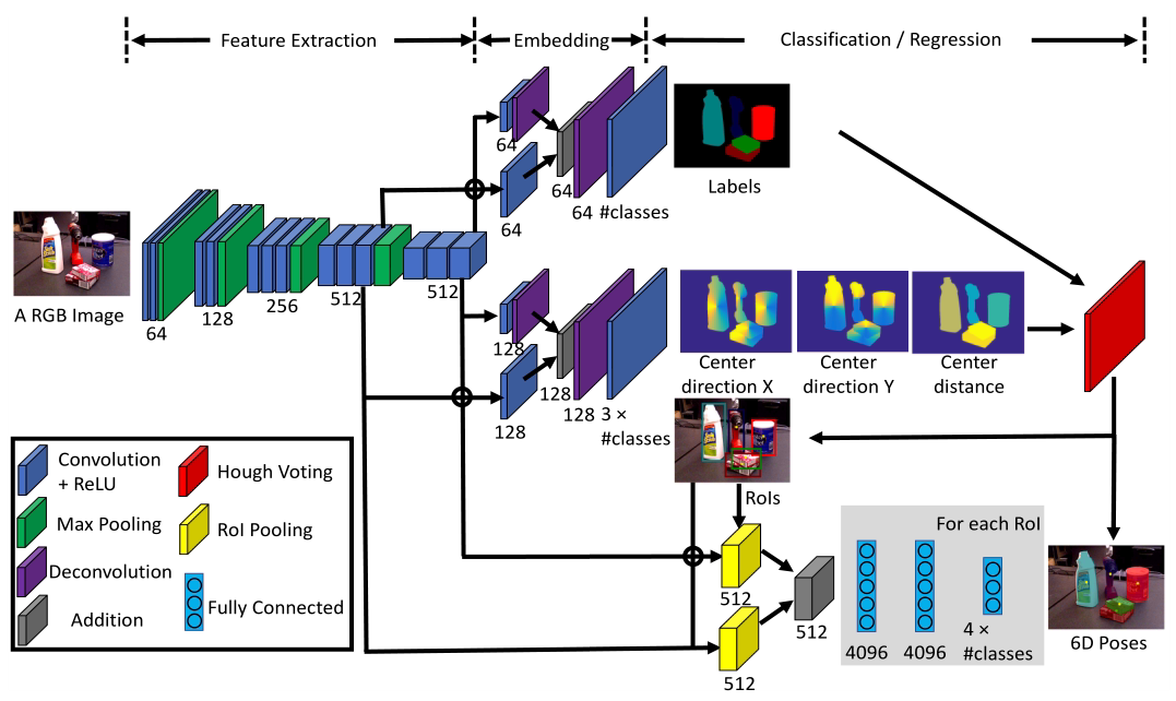
PoseCNN is mainly divided into two stages:

1. Backbone network: consists of 13 convolutional layers and 4 max-pooling layers and extracts feature maps.
2. Map the high-dimensional feature maps generated by the backbone network to a lower dimension.
3. Perform three different estimation tasks

2.2 Semantic Labels

The semantic label branch uses two feature maps, both with 512 channels, whose resolutions are reduced to 1/8 and 1/16 of the original image, respectively.

This branch first reduces the feature-map dimension to 64, then uses a deconvolution layer to double the resolution of the 1/16 image, producing two 64-channel feature maps at 1/8 resolution.

The two feature maps are then added together and passed through another deconvolution, increasing the resolution by a factor of 8 to produce a feature map the same size as the original image.

Finally, a convolutional layer is applied to the feature map to generate semantic label scores for the pixels. The output of this layer has n channels (where n is the number of semantic classes). During training, the semantic label branch is trained using Softmax cross-entropy loss; during testing, the softmax function is used to calculate the class probability for each pixel.

2.3 3D Position Estimation

(1) Principle

The 3D translation is estimated by locating the object’s center in the image and its distance from the camera.

The principle is that once the projection of T on the image, $c=(c_x, c_y)^T$, and the distance $T_z$ are known, $T_x$ and $T_y$ can be calculated.

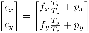
Here, $f_x$ and $f_y$ are the focal lengths, and $p_x$ and $p_y$ are the coordinates of the image principal point.

(2) Determining the Object Center

The conventional approach is to detect the center point directly, but this cannot handle cases where the object is occluded.

This paper uses the idea of an implicit shape model to regress every pixel in the image to three variables:

Here, $P=(x, y)$ is a pixel in the image, and $(c_x, c_y)$ is the coordinate of the object center. $n_x$ denotes the normalized offset between the pixel and the center point in the $x$ direction. $n_y$ denotes the offset in the y direction, and $T_z$ denotes the pixel’s predicted depth.

The variables to be predicted are therefore $(n_x, n_y, T_z)$.

Because three variables need to be regressed, a 128-channel feature map is used. The final convolutional layer has 3xn channels, where n is the number of object classes.

After obtaining the 3 variables predicted for each pixel, the coordinates of the object center need to be determined

A Hough voting mechanism is introduced, taking the pixel-level semantic label results and center regression results as input.

Each pixel votes along the ray direction predicted by the network for the location of the object center in the image. Once the pixels of all object classes have voted, all voting scores are obtained, and the position with the highest score is selected as the object-center position.

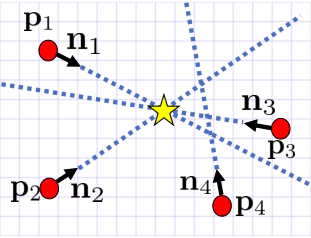
When an image contains multiple objects of the same class, non-maximum suppression is used, with a threshold set to select scores.

Through the operations above, the three-dimensional coordinates of the object center can be determined, with the predicted $T_z$ treated as the distance to the center point inside the object.

2.4 3D Orientation Estimation

(1) Network Structure

The 3D rotation estimation branch uses the ROI regions of the feature maps obtained from the backbone network and performs 3D regression through two pooling layers.

All feature maps are added together and fed into three fully connected layers. The first two fully connected layers have a dimension of 4096, and the final fully connected layer has a dimension of 4xn, where n is the number of object classes. Each object outputs a 3D rotation represented by a quaternion.

(2) Loss Function Design

Two loss functions are designed to regress the quaternion.

PoseLoss (PLoss)

It is computed in 3D space as the average squared distance between points under the correct model pose and points under the measured pose.

Here, $M$ represents a set of three-dimensional model points, m is the number of points, and $R(\overline q)$ and $R(q)$ represent the estimated rotation matrix and the ground-truth rotation matrix, respectively.

ShapeMatch-Loss (SLOSS)

Because the PLoss loss function cannot handle symmetric objects, there can be many correct three-dimensional rotation matrices for a symmetric object.

The following loss function is therefore designed:

This loss function measures the offset between points on the predicted model and their nearest points on the ground-truth model. In this way, SLoss does not penalize equivalent rotations of a symmetric object around its symmetry axis.

Note: This calculation does not require distances to be calculated in three-dimensional space. Instead, the transformed points are projected onto the image, and the distance in image space (reprojection error) is calculated.

III. Experiments

3.1 Datasets

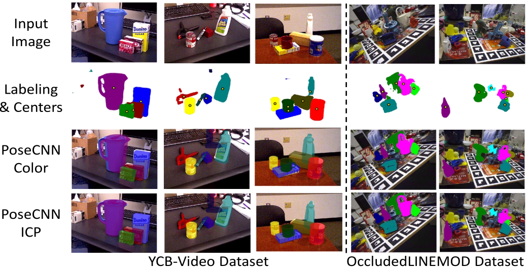
Tests are conducted on the YCB dataset and the Occluded-LINEMOD dataset (a video segment with severe object occlusion selected from the LINEMOD dataset).

3.2 Comparison Baseline

When the paper was published, mainstream pose-estimation methods regressed image pixels to 3D object coordinates. The authors therefore implemented a variant modified from the PoseCNN network that directly regresses the three-dimensional coordinates of each pixel in the object coordinate system. They removed the 3D rotation prediction branch and instead recovered the 6D pose through RANSAC using the semantic label results and the 3D object-coordinate results.

3.3 Improvement

When depth is available, the ICP algorithm is used to refine the 6D pose.

IV. PoseCNN Visualization

The original author of the following content is Panpanpan! Category: Advanced DenseFusion Article tags: deep learning PyTorch computer vision Copyright notice: This is an original article by the blogger and is licensed under the CC 4.0 BY-SA license. Please include a link to the original article and this notice when reproducing it. Article link: https://blog.csdn.net/weixin_44564705/article/details/125129844 Complete code walkthrough directory for the DenseFusion series: Complete DenseFusion Series Directory: Code Walkthrough + Visualization + Evaluation Metric Calculation — Panpanpan!‘s Blog — CSDN Blog All of this content consists of personal study notes. Please point out any errors so we can discuss and learn together!

---

Visualization Results

Select the image to visualize, enter its path, and then run eval on it to estimate the pose pred. The projections of the target point cloud and pred point cloud onto the two-dimensional image are output as follows:

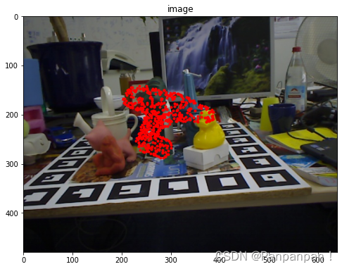
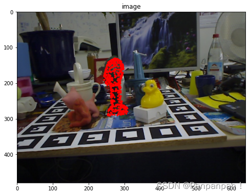
The image on the left is pred, and the one on the right is target.

Detailed Procedure

The code is located at tools/draw_linemod.py

The script is located at experiments/scripts/draw_linemod.sh

First, look at the contents of the script file:

#!/bin/bash

set -x
set -e

export PYTHONUNBUFFERED="True"
export CUDA_VISIBLE_DEVICES=0

python3 ./tools/draw_linemod.py --data_root ./datasets/linemod/Linemod_preprocessed/data/08\
  --item 0707\
  --seg_root ./datasets/linemod/Linemod_preprocessed/segnet_results/08_label\
  --obj 8\
  --model_root ./datasets/linemod/Linemod_preprocessed/models\
  --model trained_models/linemod/original/pose_model_current.pth\
  --refine_model trained_models/linemod/original/pose_refine_model_current.pth\
  --output ./

The parameters are:

 —data_root: Path to the folder for the selected image class
  —item: Number of the selected image
  —seg_root: Because this runs in eval mode, a standard segmentation label is required. Enter the semantic segmentation path for the selected image class here
  —obj: Image class number
  —model_root: Path to the image class metadata model
  —model: Path to the trained PoseNet
  —refine_model: Path to the trained PoseRefineNet

  —output: Path where visualizations are saved

Enter these parameters, then run the following in the DenseFusion folder:

./experiments/scripts/draw_linemod.sh

If this is the first time running it, you may be told that the .sh file does not have permission. Run the following command to grant permission:

chmod +x ./experiments/scripts/draw_linemod.sh

You can then view the two images in the output path.

Complete Code

 draw_linemod.py

# -*- coding: utf-8 -*-
import _init_paths
import argparse
import os
from PIL import Image
import numpy as np
import numpy.ma as ma
import torch
import random
import torchvision.transforms as transforms
import yaml
import cv2
from torch.autograd import Variable
from lib.network import PoseNet, PoseRefineNet
from lib.loss import Loss
from lib.loss_refiner import Loss_refine
from lib.knn.__init__ import KNearestNeighbor
from lib.transformations import euler_matrix, quaternion_matrix, quaternion_from_matrix
import copy
import os
from PIL import Image
import matplotlib.pyplot as plt

border_list = [-1, 40, 80, 120, 160, 200, 240, 280, 320, 360, 400, 440, 480, 520, 560, 600, 640, 680]
img_width = 480
img_length = 640
def mask_to_bbox(mask):
    mask = mask.astype(np.uint8)
    _, contours, _ = cv2.findContours(mask, cv2.RETR_TREE, cv2.CHAIN_APPROX_SIMPLE)
    
    x = 0
    y = 0
    w = 0
    h = 0
    for contour in contours:
        tmp_x, tmp_y, tmp_w, tmp_h = cv2.boundingRect(contour)
        if tmp_w * tmp_h > w * h:
            x = tmp_x
            y = tmp_y
            w = tmp_w
            h = tmp_h
    return [x, y, w, h]


def get_bbox(bbox):
    bbx = [bbox[1], bbox[1] + bbox[3], bbox[0], bbox[0] + bbox[2]]
    if bbx[0] < 0:
        bbx[0] = 0
    if bbx[1] >= 480:
        bbx[1] = 479
    if bbx[2] < 0:
        bbx[2] = 0
    if bbx[3] >= 640:
        bbx[3] = 639                
    rmin, rmax, cmin, cmax = bbx[0], bbx[1], bbx[2], bbx[3]
    r_b = rmax - rmin
    for tt in range(len(border_list)):
        if r_b > border_list[tt] and r_b < border_list[tt + 1]:
            r_b = border_list[tt + 1]
            break
    c_b = cmax - cmin
    for tt in range(len(border_list)):
        if c_b > border_list[tt] and c_b < border_list[tt + 1]:
            c_b = border_list[tt + 1]
            break
    center = [int((rmin + rmax) / 2), int((cmin + cmax) / 2)]
    rmin = center[0] - int(r_b / 2)
    rmax = center[0] + int(r_b / 2)
    cmin = center[1] - int(c_b / 2)
    cmax = center[1] + int(c_b / 2)
    if rmin < 0:
        delt = -rmin
        rmin = 0
        rmax += delt
    if cmin < 0:
        delt = -cmin
        cmin = 0
        cmax += delt
    if rmax > 480:
        delt = rmax - 480
        rmax = 480
        rmin -= delt
    if cmax > 640:
        delt = cmax - 640
        cmax = 640
        cmin -= delt
    return rmin, rmax, cmin, cmax
def ply_vtx(path):
    f = open(path)
    assert f.readline().strip() == "ply"
    f.readline()
    f.readline()
    N = int(f.readline().split()[-1])
    while f.readline().strip() != "end_header":
        continue
    pts = []
    for _ in range(N):
        pts.append(np.float32(f.readline().split()[:3]))
    return np.array(pts)

def get_data(data_root, item, seg_root, obj, model_root, add_noise, noise_trans):
    img = Image.open('{0}/rgb/{1}.png'.format(data_root, item))
    ori_img = np.array(img)
    depth = np.array(Image.open('{0}/depth/{1}.png'.format(data_root, item)))
    label = np.array(Image.open('{0}/{1}_label.png'.format(seg_root, item)))
    print('{0}/depth/{1}.png'.format(data_root, item))
    print('{0}/{1}_label.png'.format(seg_root, item))
    print('{0}/gt.yml'.format(data_root))
    print('{0}/obj_{1}.ply'.format(model_root, '%02d' % obj))
    
    meta_file = open('{0}/gt.yml'.format(data_root), 'r')
    meta = yaml.load(meta_file, Loader=yaml.FullLoader)
    pt = ply_vtx('{0}/obj_{1}.ply'.format(model_root, '%02d' % obj))
    
    trancolor = transforms.ColorJitter(0.2, 0.2, 0.2, 0.05)
    norm = transforms.Normalize(mean=[0.485, 0.456, 0.406], std=[0.229, 0.224, 0.225])
    num = 500
    xmap = np.array([[j for i in range(640)] for j in range(480)])
    ymap = np.array([[i for i in range(640)] for j in range(480)])
    cam_cx = 325.26110
    cam_cy = 242.04899
    cam_fx = 572.41140
    cam_fy = 573.57043
    num_pt_mesh_large = 500
    num_pt_mesh_small = 500
    rank = int(item)
    if obj == 2:
        for i in range(0, len(meta[obj])):
            if meta[rank][i]['obj_id'] == 2:
                meta = meta[rank][i]
                break
    else:
        meta = meta[rank][0]

    mask_depth = ma.getmaskarray(ma.masked_not_equal(depth, 0))
    mask_label = ma.getmaskarray(ma.masked_equal(label, np.array(255)))
    mask = mask_label * mask_depth

    if add_noise:
        img = trancolor(img)

    img = np.array(img)[:, :, :3]
    img = np.transpose(img, (2, 0, 1))
    img_masked = img

    rmin, rmax, cmin, cmax = get_bbox(mask_to_bbox(mask_label))
    img_masked = img_masked[:, rmin:rmax, cmin:cmax]
    #p_img = np.transpose(img_masked, (1, 2, 0))
    #scipy.misc.imsave('evaluation_result/{0}_input.png'.format(index), p_img)

    target_r = np.resize(np.array(meta['cam_R_m2c']), (3, 3))
    target_t = np.array(meta['cam_t_m2c'])
    add_t = np.array([random.uniform(-noise_trans, noise_trans) for i in range(3)])

    choose = mask[rmin:rmax, cmin:cmax].flatten().nonzero()[0]
    if len(choose) == 0:
        cc = torch.LongTensor([0])
        return(cc, cc, cc, cc, cc, cc)

    if len(choose) > num:
        c_mask = np.zeros(len(choose), dtype=int)
        c_mask[:num] = 1
        np.random.shuffle(c_mask)
        choose = choose[c_mask.nonzero()]
    else:
        choose = np.pad(choose, (0, num - len(choose)), 'wrap')
    
    depth_masked = depth[rmin:rmax, cmin:cmax].flatten()[choose][:, np.newaxis].astype(np.float32)
    xmap_masked = xmap[rmin:rmax, cmin:cmax].flatten()[choose][:, np.newaxis].astype(np.float32)
    ymap_masked = ymap[rmin:rmax, cmin:cmax].flatten()[choose][:, np.newaxis].astype(np.float32)
    choose = np.array([choose])

    cam_scale = 1.0
    pt2 = depth_masked / cam_scale
    pt0 = (ymap_masked - cam_cx) * pt2 / cam_fx
    pt1 = (xmap_masked - cam_cy) * pt2 / cam_fy
    cloud = np.concatenate((pt0, pt1, pt2), axis=1)
    cloud = cloud / 1000.0
    print(cloud.shape)

    if add_noise:
        cloud = np.add(cloud, add_t)

    #fw = open('evaluation_result/{0}_cld.xyz'.format(index), 'w')
    #for it in cloud:
    #    fw.write('{0} {1} {2}\n'.format(it[0], it[1], it[2]))
    #fw.close()
    model_points = pt/ 1000.0
    dellist = [j for j in range(0, len(model_points))]
    dellist = random.sample(dellist, len(model_points) - num_pt_mesh_small)
    model_points = np.delete(model_points, dellist, axis=0)

    #fw = open('evaluation_result/{0}_model_points.xyz'.format(index), 'w')
    #for it in model_points:
    #    fw.write('{0} {1} {2}\n'.format(it[0], it[1], it[2]))
    #fw.close()

    target = np.dot(model_points, target_r.T)
    if add_noise:
        target = np.add(target, target_t / 1000.0 + add_t)
        out_t = target_t / 1000.0 + add_t
    else:
        target = np.add(target, target_t / 1000.0)
        out_t = target_t / 1000.0

    #fw = open('evaluation_result/{0}_tar.xyz'.format(index), 'w')
    #for it in target:
    #    fw.write('{0} {1} {2}\n'.format(it[0], it[1], it[2]))
    #fw.close()

    return torch.from_numpy(cloud.astype(np.float32)), \
           torch.LongTensor(choose.astype(np.int32)), \
           norm(torch.from_numpy(img_masked.astype(np.float32))), \
           torch.from_numpy(target.astype(np.float32)), \
           torch.from_numpy(model_points.astype(np.float32)), \
           torch.LongTensor([obj])


parser = argparse.ArgumentParser()
parser.add_argument('--data_root', type=str, default = '', help='ycb or linemod')
parser.add_argument('--seg_root', type=str, default = '', help='ycb or linemod')
parser.add_argument('--model_root', type=str, default = '', help='ycb or linemod')
parser.add_argument('--item', type=str, default = '', help='')
parser.add_argument('--obj', type=int, default=1, help='')
parser.add_argument('--model', type=str, default = '',  help='resume PoseNet model')
parser.add_argument('--refine_model', type=str, default = '',  help='resume PoseRefineNet model')
parser.add_argument('--output', type=str, default = '',  help='resume PoseRefineNet model')
opt = parser.parse_args() 


estimator = PoseNet(num_points = 500, num_obj = 13)
estimator.cuda()
refiner = PoseRefineNet(num_points = 500, num_obj = 13)
refiner.cuda()
estimator.load_state_dict(torch.load(opt.model))
refiner.load_state_dict(torch.load(opt.refine_model))

bs = 1
num_points = 500
iteration = 4
knn = KNearestNeighbor(1)

for i in range(1):
    points, choose, img, target, model_points, idx = get_data(opt.data_root, opt.item, opt.seg_root, opt.obj, opt.model_root, True, 0.0)
  
    if len(points.size()) == 1:
        print('No.{0} NOT Pass! Lost detection!'.format(i))
        continue
    points, choose, img, target, model_points, idx = Variable(points.unsqueeze(0)).cuda(), \
                                                        Variable(choose.unsqueeze(0)).cuda(), \
                                                        Variable(img.unsqueeze(0)).cuda(), \
                                                        Variable(target.unsqueeze(0)).cuda(), \
                                                        Variable(model_points.unsqueeze(0)).cuda(), \
                                                        Variable(idx.unsqueeze(0)).cuda()
    pred_r, pred_t, pred_c, emb = estimator(img, points, choose, idx)
    pred_r = pred_r / torch.norm(pred_r, dim=2).view(1, num_points, 1)
    pred_c = pred_c.view(bs, num_points)
    how_max, which_max = torch.max(pred_c, 1)
    pred_t = pred_t.view(bs * num_points, 1, 3)

    my_r = pred_r[0][which_max[0]].view(-1).cpu().data.numpy()
    my_t = (points.view(bs * num_points, 1, 3) + pred_t)[which_max[0]].view(-1).cpu().data.numpy()
    my_pred = np.append(my_r, my_t)
    for ite in range(0, iteration):
        Tt = Variable(torch.from_numpy(my_t.astype(np.float32))).cuda().view(1, 3).repeat(num_points, 1).contiguous().view(1, num_points, 3)
        my_mat = quaternion_matrix(my_r)
        R = Variable(torch.from_numpy(my_mat[:3, :3].astype(np.float32))).cuda().view(1, 3, 3)
        my_mat[0:3, 3] = my_t
        
        new_points = torch.bmm((points - Tt), R).contiguous()
        pred_r, pred_t = refiner(new_points, emb, idx)
        pred_r = pred_r.view(1, 1, -1)
        pred_r = pred_r / (torch.norm(pred_r, dim=2).view(1, 1, 1))
        my_r_2 = pred_r.view(-1).cpu().data.numpy()
        my_t_2 = pred_t.view(-1).cpu().data.numpy()
        my_mat_2 = quaternion_matrix(my_r_2)
        my_mat_2[0:3, 3] = my_t_2

        my_mat_final = np.dot(my_mat, my_mat_2)
        my_r_final = copy.deepcopy(my_mat_final)
        my_r_final[0:3, 3] = 0
        my_r_final = quaternion_from_matrix(my_r_final, True)
        my_t_final = np.array([my_mat_final[0][3], my_mat_final[1][3], my_mat_final[2][3]])

        my_pred = np.append(my_r_final, my_t_final)
        my_r = my_r_final
        my_t = my_t_final
    model_points = model_points[0].cpu().detach().numpy()
    my_r = quaternion_matrix(my_r)[:3, :3]
    pred = np.dot(model_points, my_r.T) + my_t  
    target = target[0].cpu().detach().numpy()

    pred = pred*1000.0
    target = target*1000.0
    cam_scale = 1.0
    cam_cx = 325.26110
    cam_cy = 242.04899
    cam_fx = 572.41140
    cam_fy = 573.57043

    depth_masked =  pred[:,2] * cam_scale
    ymap_masked_pred =  pred[:,0] * cam_fx / pred[:,2] + cam_cx
    xmap_masked_pred = pred[:,1] * cam_fy / pred[:,2] + cam_cy

    depth_masked =  target[:,2] * cam_scale
    ymap_masked_target =  target[:,0] * cam_fx / target[:,2] + cam_cx
    xmap_masked_target = target[:,1] * cam_fy / target[:,2] + cam_cy

    image = Image.open('{0}/rgb/{1}.png'.format(opt.data_root, opt.item))

    plt.figure(figsize=(8,12)) # 图像窗口名称
    plt.imshow(image)
    plt.scatter(ymap_masked_pred,xmap_masked_pred,marker='.',c='r',alpha=1)
    plt.axis('on') # 关掉坐标轴为 off
    plt.title('image') # 图像题目
    plt.show()  
    plt.savefig('{0}/test_pred.png'.format(opt.output))

    plt.figure(figsize=(8,12)) # 图像窗口名称
    plt.imshow(image)
    plt.scatter(ymap_masked_target,xmap_masked_target,marker='.',c='r',alpha=1)
    plt.axis('on') # 关掉坐标轴为 off
    plt.title('image') # 图像题目
    plt.show() 
    plt.savefig('{0}/test_target.png'.format(opt.output))