[6D Pose Estimation] Gen6D Algorithm

Paper Notes

Title: Gen6D: Generalizable Model-Free 6-DoF Object Pose Estimation from RGB Images Authors: The University of Hong Kong Venue: ECCV Year: 2022 Code: https://github.com/liuyuan-pal/Gen6D

1. Introduction

1.1 Problem Statement

Existing pose estimation methods either require high-quality object models or additional depth maps or object mask images, which greatly limits practical deployment. The method proposed in this paper needs only a set of posed reference images of an object and can predict the object pose in arbitrary environments.

The authors argue that a pose estimator should have the following properties:

• Generalizability: applicable to arbitrary objects without training on specific objects or categories
• Model-free: for an unseen object, only a few reference images with known poses are needed to define the object reference frame
• Simple input: estimate pose from RGB images only, without depth maps or object masks

(1) How to design a viewpoint selector that finds the reference image whose viewpoint is closest to the query image

This paper uses a neural network to compare the query image and reference images pixel by pixel, produce similarity scores, and select the reference image with the highest score. It also adds a global normalization layer and a self-attention layer to share similarity information across different reference images, providing contextual information for selecting the most similar reference image.

(2) Achieving model-free pose refinement

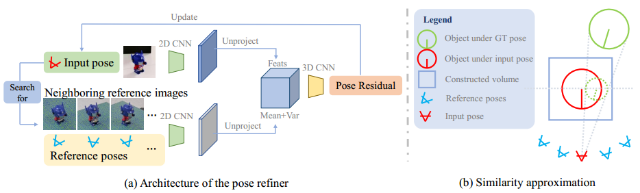
This paper proposes a new pose refinement method based on three-dimensional space. Given a query image and an input pose, it finds several reference images close to that pose, projects them back into 3D space to build a feature space, and refines the pose by matching that feature space with query-image features through a 3D CNN.

1.2 Related Work

Most existing pose estimation methods are instance-specific and do not generalize to unseen objects. They usually require rendering large numbers of images from a 3D object model for training. Some methods generalize to the category level and do not require object models, but they still cannot predict objects from unseen categories.

2. Method

Data normalization: For each object, the authors estimate the object’s approximate size from the reference images using methods such as triangulation, then normalize the object coordinate frame so that the object center lies at the origin and its size is 1. The object then lies inside the unit sphere centered at the origin.

Gen6D consists of an object detector, a viewpoint selector, and a pose refiner.

The object detector first uses the query image and reference images to detect the object region. The viewpoint selector then matches the query image with reference images to produce a coarse initial pose. Finally, the pose refiner further refines it to obtain an accurate object pose.

2.1 Object Detection

The detection problem is decomposed into two parts:

1. Find the 2D projection point q of the object center
2. Estimate the square bounding box that encloses the unit sphere

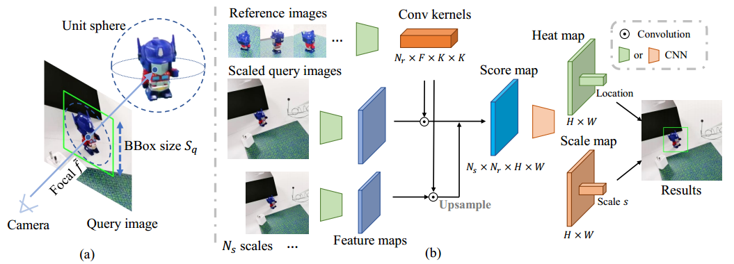
The depth of the object center can be computed as $d=2f/S_q$, where 2 is the diameter of the unit sphere, f is the virtual focal length (with the principal point set to projection point q), and $S_q$ is the side length of the bounding box. This gives the initial translation of the object.

Question: After normalizing the object, is the depth d computed here still the real depth? How is the virtual focal length determined?

The detector uses a VGG network to extract feature maps from the reference images and the query image, then uses all reference-image feature maps as convolution kernels to convolve with the query-image feature map and obtain a score map. To account for scale differences, convolutions are performed at multiple predefined scales, producing a heatmap and a scale map. The maximum location on the heatmap is chosen as the 2D projection of the object center, and the scale at the same location on the scale map is used as the bounding-box size $S_q=S_r*s$.

Question: Since feature maps from all reference images are convolved, how are object features and background features in the reference images distinguished?

2.2 Viewpoint Selection

The query image is compared with each reference image to compute a similarity score. The element-wise product of each reference image and the query image yields a score map, from which similarity parameters are computed.

(1) In-plane rotation To account for in-plane rotation, the paper rotates each reference image by Na predefined angles and uses all rotated versions for element-wise multiplication during querying.

(2) Global normalization The feature maps produced by the similarity network are normalized using the mean and variance computed from all reference-image feature maps. This encodes contextual similarity through the distribution of feature maps and amplifies similarity differences across images.

(3) Reference-viewpoint transformation A transformation—including their viewpoints and attention layers—is applied to the similarity feature vectors of all reference images. This transformer lets feature vectors communicate with one another to encode contextual information, which helps determine the most similar reference image.

2.3 Pose Refinement

After the two steps above, we already have a coarse object pose. This step refines the pose.

6 reference images close to the input pose are selected. A CNN extracts feature maps, which are projected into 3D space. The mean and variance of the features are computed as the feature at each spatial vertex. For the query image, the same CNN extracts feature maps, projects them into 3D space, and concatenates the query features with the mean and variance of the reference-image features.

Finally, a 3D CNN on the spatial features predicts residuals to update the input pose.

3. Experimental Analysis

II. Algorithm Reproduction

2.1 Environment Setup

2.1.1 Python Environment

Create an Anaconda virtual environment

conda create -n gen6d python=3.7
conda activate gen6d

Install the PyTorch environment

conda install pytorch==1.7.1 torchvision==0.8.2 torchaudio==0.7.2 -c pytorch

Install dependencies. Open requirements.txt and remove pytorch, torchvision, and cudatoolkit from it.

pip install -r requirements.txt

2.1.2 Custom Dataset Tools

(1) COLMAP

Follow the official tutorial: https://colmap.github.io/install.html

Install dependencies

sudo apt-get install \
    git \
    cmake \
    build-essential \
    libboost-program-options-dev \
    libboost-filesystem-dev \
    libboost-graph-dev \
    libboost-regex-dev \
    libboost-system-dev \
    libboost-test-dev \
    libeigen3-dev \
    libsuitesparse-dev \
    libfreeimage-dev \
    libgoogle-glog-dev \
    libgflags-dev \
    libglew-dev \
    qtbase5-dev \
    libqt5opengl5-dev \
    libcgal-dev \
    libcgal-qt5-dev\
    libceres-dev\
    ninja-build\
    libmetis-dev

Download the COLMAP source code

git clone https://github.com/colmap/colmap
cd colmap

Edit the CMakeLists.txt file and add the following content

set(CMAKE_CUDA_ARCHITECTURES 86)

Build and install (make sure to exit the conda environment before building and installing)

mkdir build
cd build
cmake .. -GNinja
ninja
sudo ninja install

(2) CloudCompare

Method 1: snap (recommended)

Install snap

sudo apt-get install snap

Install CloudCompare

snap install cloudcompare

Launch CloudCompare

cloudcompare.CloudCompare

Method 2: Flatpak

Install Flatpak

sudo apt install flatpak

Install the Software Flatpak plugin

sudo apt install gnome-software-plugin-flatpak

Add the Flathub repository

flatpak remote-add --if-not-exists flathub https://flathub.org/repo/flathub.flatpakrepo

Install CloudCompare

flatpak install flathub org.cloudcompare.CloudCompare

Run CloudCompare

flatpak run org.cloudcompare.CloudCompare

(3) Install ffmpeg

sudo apt install ffmpeg

2.2 Dataset Preparation

2.2.1 Official Datasets

(1) Download datasets

Download the pretrained models, GenMOP dataset, and processed LINEMOD dataset from the link provided by the authors.

(2) Organize the datasets

Organize the downloaded files in the following structure.

Gen6D
|-- data
    |-- model
        |-- detector_pretrain
            |-- model_best.pth
        |-- selector_pretrain
            |-- model_best.pth
        |-- refiner_pretrain
            |-- model_best.pth
    |-- GenMOP
        |-- chair 
            ...
    |-- LINEMOD
        |-- cat 
            ...

2.2.2 Custom Datasets

(1) Video recording

Use a phone to record reference and test videos of the target object. Note: the reference video must satisfy the following conditions:

• The object is static in the reference video
• The background in the reference video should be as textured and flat as possible, and the camera should cover as many viewpoints as possible so that COLMAP can recover camera poses

(2) Organize files

Organize the videos in the following paths

Gen6D
|-- data
    |-- custom
       |-- video
           |-- mouse-ref.mp4
           |-- mouse-test.mp4

(3) Split the reference video into images

## 每10帧保存一张图像，最大图像边长为960
python prepare.py --action video2image \
                  --input data/custom/video/ref/realsensebox-ref.mp4 \
                  --output data/custom/realsensebox/images \
                  --frame_inter 10 \
                  --image_size 960 \
                  --transpose
## 或者
python prepare.py --action video2image --input data/custom/video/ammeter-ref.mp4 --output data/custom/ammeter/images --frame_inter 10 --image_size 960 --transpose

The split video is saved in data/custom/coffeebox/images.

(4) Run COLMAP SfM to recover camera poses

python prepare.py --action sfm --database_name custom/realsensebox --colmap /usr/local/bin/colmap

Note: you can find <path-to-your-colmap-exe> with the command which colmap. On Ubuntu it is usually /usr/local/bin/colmap; on Windows it is E:/Programming/COLMAP-3.8-windows-cuda/COLMAP.bat

(5) Manually process the point cloud

Manually determine the object region by cropping the object point cloud. For example, use CloudCompare to visualize and process the point cloud reconstructed by COLMAP. The reconstructed point cloud is located at data/custom/mouse/colmap/pointcloud.ply.

flatpak run org.cloudcompare.CloudCompare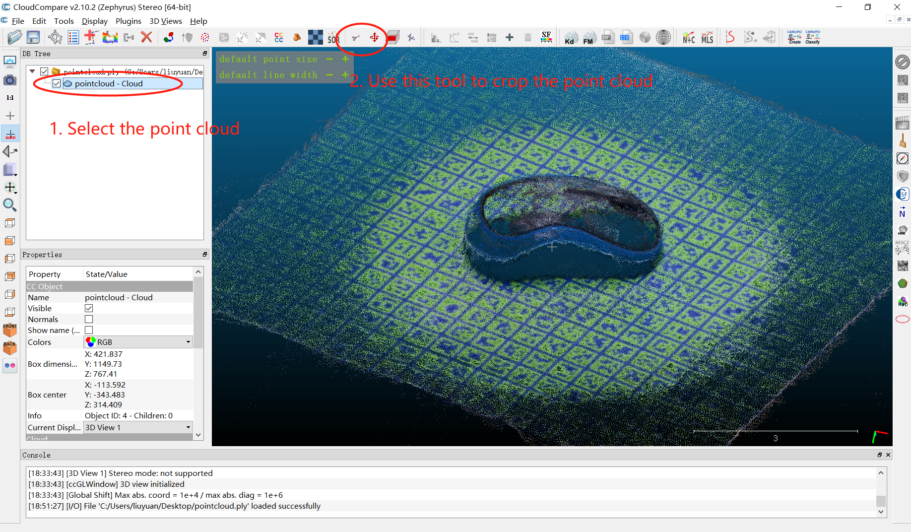

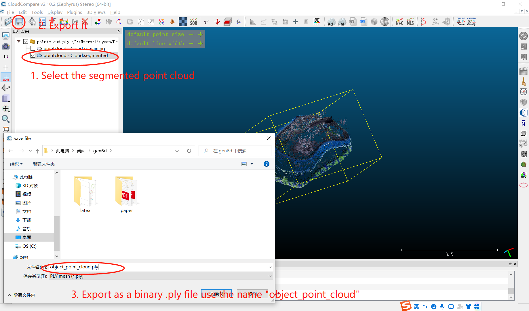
Export the cropped point cloud as data/custom/mouse/object_point_cloud.ply.

(6) Manually determine the positive X-axis and positive Z-axis of the object

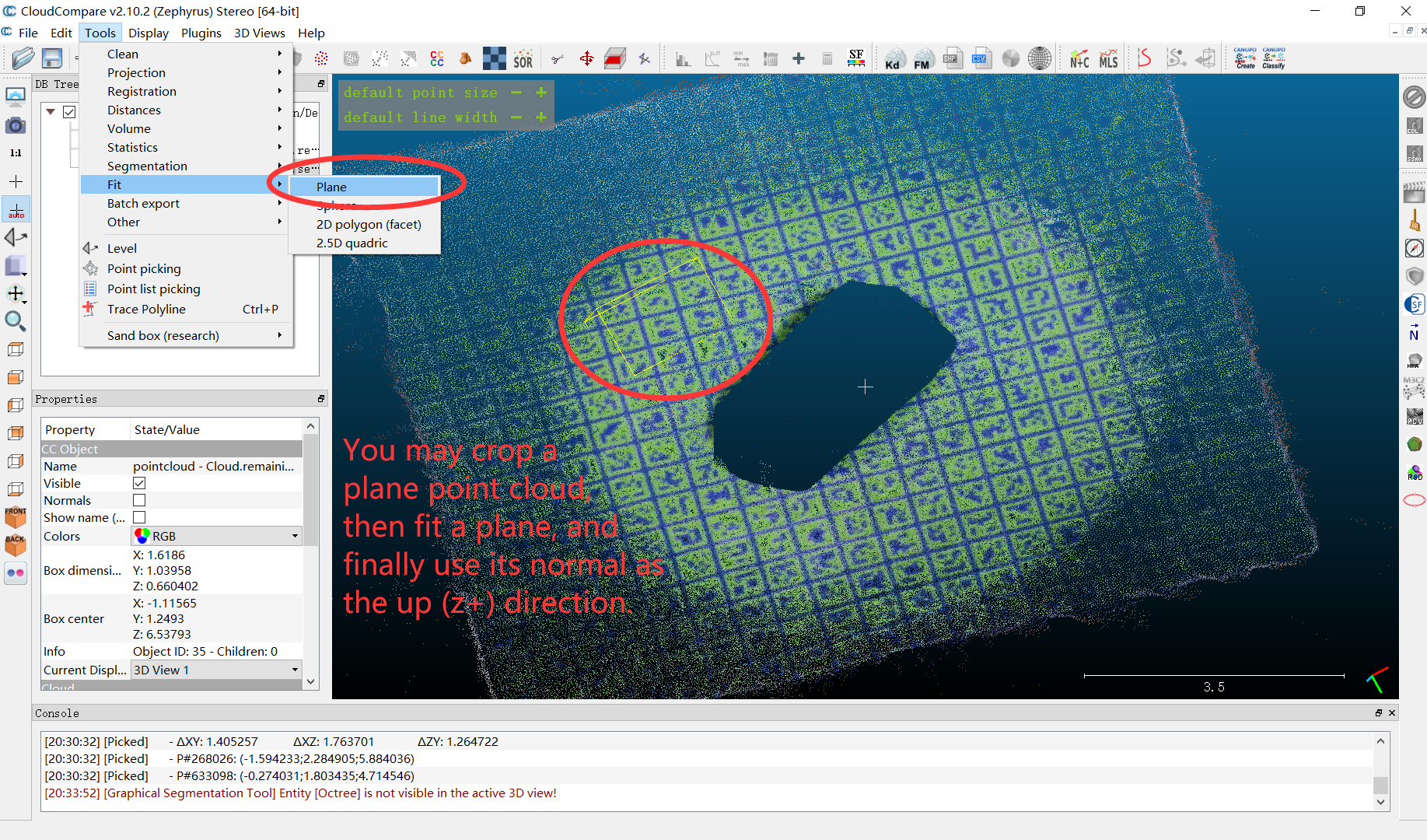
Edit a data/custom/mouse/meta_info.txt file to save your X+ and Z+ information, for example

2.297052 0.350839 -0.000593
0.973488 0.054352 -0.222188

(7) Make sure you have the following files generated by the steps above

Gen6D
|-- data
    |-- custom
       |-- mouse
           |-- object_point_cloud.ply  ## object point cloud
           |-- meta_info.txt           ## meta information about z+/x+ directions
           |-- images                  ## images
           |-- colmap                  ## colmap project

(8) Predict poses from the processed reference images

python predict.py --cfg configs/gen6d_pretrain.yaml \
                  --database custom/realsensebox \
                  --video data/custom/video/test/realsensebox-test.mp4 \
                  --resolution 1280 \
                  --transpose \
                  --output data/custom/video/test \
                  --ffmpeg <path-to-ffmpeg-exe>

2.3 Training and Evaluation

Download the processed co3d data (co3d.tar.gz), Google Scanned Objects data (google_scanned_objects.tar.gz), and ShapeNet renders (shapenet.tar.gz), plus the pretrained models (gen6d_pretrain.tar.gz), from here.

Download COCO 2017 Train images

Organize the files as follows

Gen6D
|-- data
    |-- custom
        |-- coffebox 
            ...
    |-- model
        |-- detector_pretrain
            |-- model_best.pth
        |-- selector_pretrain
            |-- model_best.pth
        |-- refiner_pretrain
            |-- model_best.pth
    |-- shapenet
        |-- shapenet_cache
        |-- shapenet_render
        |-- shapenet_render_v1.pkl
    |-- co3d_256_512
        |-- apple
            ...
    |-- google_scanned_objects
        |-- 06K3jXvzqIM
            ...
    |-- coco
        |-- train2017

2.3.1 Train the detector

Edit line 86 of train_meta_info.py

'genmop_train': [f'genmop/{name}-test' for name in ['ammeter', 'coffeebox', 'realsensebox']],

Edit line 109 of database.py

GenMOP_ROOT = 'data/custom'

genmop_meta_info={
    'ammeter': {'gravity': np.asarray([0.0222805, -0.409031, 0.912248]), 'forward': np.asarray([0.401556, 0.773825, 0.340199],np.float32)},
    'coffeebox': {'gravity': np.asarray([0.0718405, -0.471545, 0.878911]), 'forward': np.asarray([0.582604, -0.490501, -0.219265],np.float32)},
    'realsensebox': {'gravity': np.asarray([0.103463, -0.521284, 0.847088],np.float32), 'forward': np.asarray([-1.690831, 0.688506, 0.590004],np.float32)},
}

Edit line 212 of database.py to

cameras, images, points3d = read_model(f'{GenMOP_ROOT}/{seq_name}/colmap/sparse/0')

Start training

python train_model.py --cfg configs/detector/detector_train.yaml

2.3.2 Train the selector

python train_model.py --cfg configs/selector/selector_train.yaml

2.3.3 Train the refiner

Prepare data for refiner training

python prepare.py --action gen_val_set \
                  --estimator_cfg configs/gen6d_train.yaml \
                  --que_database linemod/cat \
                  --que_split linemod_val \
                  --ref_database linemod/cat \
                  --ref_split linemod_val

python prepare.py --action gen_val_set \
                  --estimator_cfg configs/gen6d_train.yaml \
                  --que_database genmop/tformer-test \
                  --que_split all \
                  --ref_database genmop/tformer-ref \
                  --ref_split all 

This command generates information in data/val, which is used to create valid data for the refiner.

Train the refiner

python train_model.py --cfg configs/refiner/refiner_train.yaml

2.3.4 Evaluate all components

# Evaluate on the object TFormer from the GenMOP dataset
python eval.py --cfg configs/gen6d_train.yaml --object_name genmop/tformer

# Evaluate on the object cat from the LINEMOD dataset
python eval.py --cfg configs/gen6d_train.yaml --object_name linemod/cat

III. Current Issues

Advantages

1. You only need to record a video of (1-2) minutes for a given object and spend (1-2) hours with the program adding the dataset to enable pose estimation for a new object, without retraining the network
2. Accuracy is acceptable

Disadvantages

1. Recognition works well for square convex objects, but poorly for objects with hollow interior regions, such as rings
2. Because the reference video requires the object to remain still, the underside cannot be captured, so recognition of the bottom surface is poor (you can place the object face up and face down for two recordings and use two reference videos for the same object, then choose the pose with higher confidence)
3. During recognition, if the object is not present in the image, the method still outputs an estimated pose (you can consider judging the output by confidence, or using algorithms such as YOLO to pre-detect the object location before pose estimation)
4. Pose estimation performs poorly under occlusion. It may box only the unoccluded part, or force pose estimation on the occluding object.
5. When many objects must be recognized at once, GPU memory requirements are high and computation becomes slow, the server 1.5s/it. If you recognize only one specific object at a time, the speed is acceptable.